counts <- matrix(
  rpois(16, lambda=100), ncol=4,
  dimnames=list(c("g1","g2","g3","g4"),
                c("s1","s2","s3","s4"))
)
counts
s1 s2 s3 s4
g1 94 117 112 94
g2 111 104 103 112
g3 83 87 104 108
g4 101 82 101 99Dept of Genetics, Dept of Biostatistics, UNC-Chapel Hill
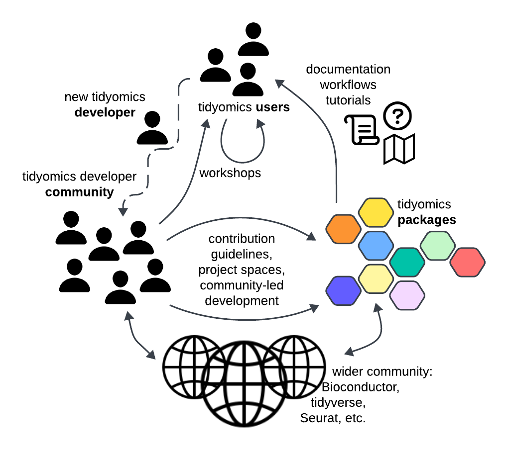
An open, open-source project spanning multiple R packages, and developers from around the world. Operates within the Bioconductor Project, with separate funding and organization. Coordination of development via GitHub Projects.
#tidiness_in_bioc channel in Zulip
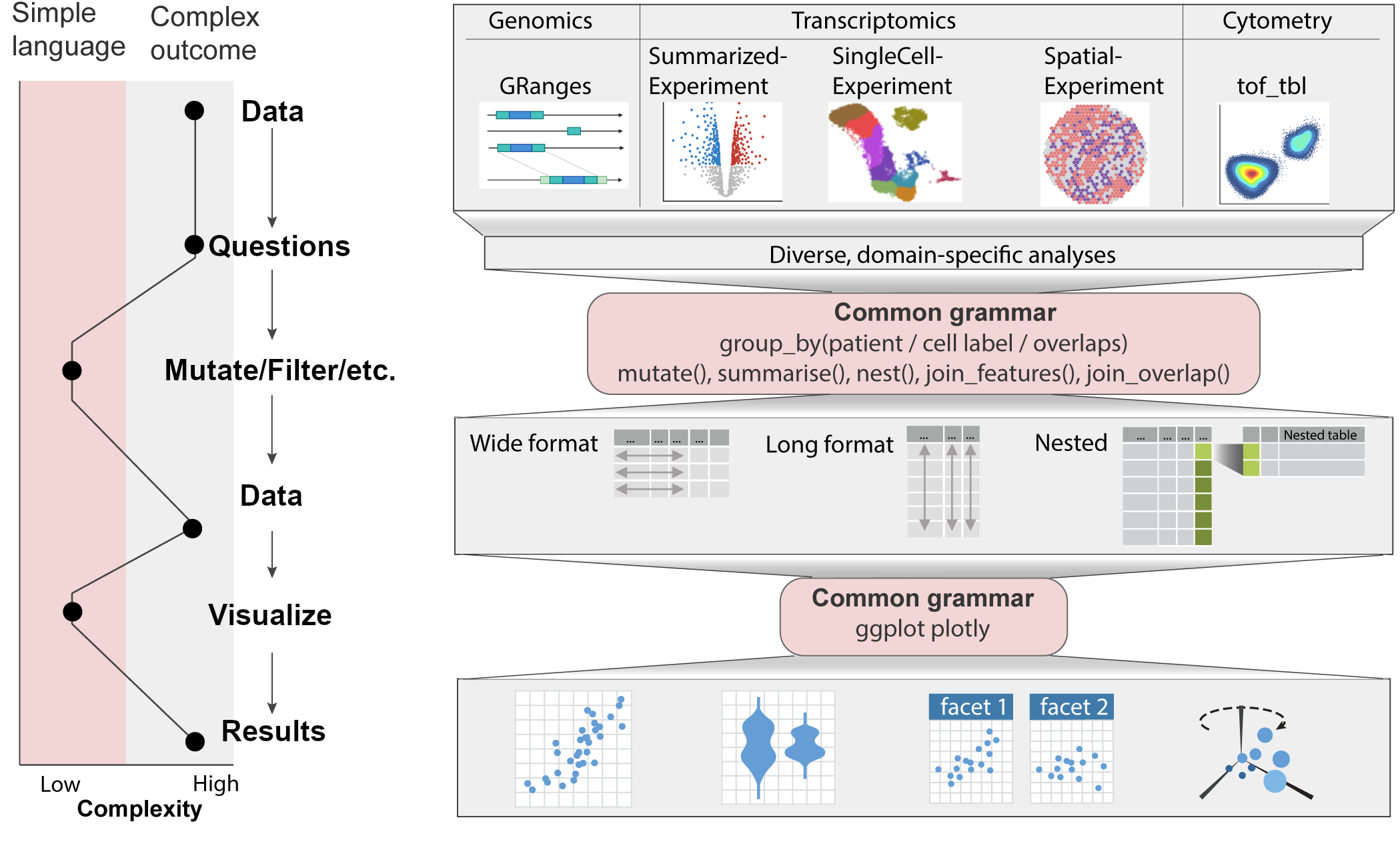
One row per observation, one column per variable.
Genomic regions (BED) already in this format.
Matrices and annotated matrices are not.
In the R package dplyr:
mutate() adds new variables that are functions of existing variables.select() picks variables based on their names.filter() picks cases based on their values.slice() picks cases based on their position.summarize() reduces multiple values down to a single summary.arrange() changes the ordering of the rows.group_by() perform any operation by group.“Pipes rank alongside the hierarchical file system and regular expressions as one of the most powerful yet elegant features of Unix-like operating systems.”
http://www.linfo.org/pipe.html
In R we use %>% or |> instead of | to chain operations.
Genomic regions (called “ranges”)
Matrix data, e.g. gene expression over samples or cells
Genomic interactions, e.g. DNA loops
And more…
We typically have more information than just a matrix
Row and column information (on features and samples)
Annotated matrix data, i.e. python’s xarray, AnnData
Metadata: organism, genome build, annotation release
2002: ExpressionSet; 2011: SummarizedExperiment
Endomorphic functions: x |> f -> x
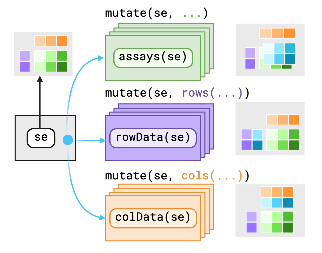
A SummarizedExperiment is annotated matrix data.
Imagine a matrix of counts:
metadata about genes (rows)
DataFrame with 4 rows and 2 columns
           id      symbol
  <character> <character>
1          g1         ABC
2          g2         DEF
3          g3         GHI
4          g4         JKL
metadata about samples (columns)
DataFrame with 4 rows and 3 columns
       sample   condition         sex
  <character> <character> <character>
1          s1           x           m
2          s2           y           m
3          s3           x           f
4 s4 y fse <- SummarizedExperiment(
assays = list(counts = counts),
rowData = genes,
colData = samples,
metadata = list(organism="Hsapiens")
)
seclass: SummarizedExperiment
dim: 4 4
metadata(1): organism
assays(1): counts
rownames(4): g1 g2 g3 g4
rowData names(2): id symbol
colnames(4): s1 s2 s3 s4
colData names(3): sample condition sexReordering columns propagates to assay and colData:
Assignment with conflicting metadata gives an error:
Other such validity checks include comparison across different genome builds.
Errors triggered by metadata better than silent errors!
[1] "colData" "assays" "NAMES" "elementMetadata" "metadata" [1] "!=,ANY,Vector-method" "!=,Vector,ANY-method"
[3] "!=,Vector,Vector-method" "[,SummarizedExperiment,ANY,ANY,ANY-method"
[5] "[[,SummarizedExperiment,ANY,missing-method" "[[<-,SummarizedExperiment,ANY,missing-method"An advanced R/Bioconductor user should eventually learn these methods, class/method inheritance.
Not needed to explore or visualize data, or make basic data summaries.
tidySummarizedExperiment package from Mangiola et al.
Printing says: “SummarizedExperiment-tibble abstraction”
# A SummarizedExperiment-tibble abstraction: 16 × 8
# Features=4 | Samples=4 | Assays=counts
   .feature .sample counts sample condition sex   id    symbol
   <chr>    <chr>    <int> <chr>  <chr>     <chr> <chr> <chr>
 1 g1       s1          94 s1     x         m     g1    ABC
 2 g2       s1         111 s1     x         m     g2    DEF
 3 g3       s1          83 s1     x         m     g3    GHI
 4 g4       s1         101 s1     x         m     g4    JKL
 5 g1       s2         117 s2     y         m     g1    ABC
 6 g2       s2         104 s2     y         m     g2    DEF
 7 g3       s2          87 s2     y         m     g3    GHI
 8 g4       s2          82 s2     y         m     g4    JKL
 9 g1       s3         112 s3     x         f     g1    ABC
10 g2       s3         103 s3     x         f     g2    DEF
11 g3       s3         104 s3     x         f     g3    GHI
12 g4       s3         101 s3     x         f     g4    JKL
13 g1       s4          94 s4     y         f     g1    ABC
14 g2       s4         112 s4     y         f     g2    DEF
15 g3       s4         108 s4     y         f     g3    GHI
16 g4 s4 99 s4 y f g4 JKL Interact with native objects using standard R/Bioc methods.
# A SummarizedExperiment-tibble abstraction: 8 × 8
# Features=4 | Samples=2 | Assays=counts
  .feature .sample counts sample condition sex   id    symbol
  <chr>    <chr>    <int> <chr>  <chr>     <chr> <chr> <chr>
1 g1       s1          94 s1     x         m     g1    ABC
2 g2       s1         111 s1     x         m     g2    DEF
3 g3       s1          83 s1     x         m     g3    GHI
4 g4       s1         101 s1     x         m     g4    JKL
5 g1       s3         112 s3     x         f     g1    ABC
6 g2       s3         103 s3     x         f     g2    DEF
7 g3       s3         104 s3     x         f     g3    GHI
8 g4 s3 101 s3 x f g4 JKL SingleCellExperiment has slots for e.g. reduced dimensions.
plyxpJustin Landis (UNC BCB) noticed some opportunities for more efficient operations.
Also, reduce ambiguity, allow multiple ways to access data across context. Leveraging data masks from rlang.
Developed in Summer 2024: plyxp, stand-alone but also as a tidySummarizedExperiment engine.
plyxpnew_plyxp()# A SummarizedExperiment-tibble Abstraction: 3 × 4
.features .samples | counts | length | type
<chr> <chr> | <int> | <dbl> | <fct>
1 A a | 1 | 10 | 1
2 B a | 2 | 20 | 1
3 C a | 3 | 30 | 1
4 A b | 4 | 10 | 1
5 B b | 5 | 20 | 1
… … … … … …
n-4 B c | 8 | 20 | 2
n-3 C c | 9 | 30 | 2
n-2 A d | 10 | 10 | 2
n-1 B d | 11 | 20 | 2
n C d | 12 | 30 | 2
# ℹ n = 12plyxp# A SummarizedExperiment-tibble Abstraction: 3 × 4
.features .samples | counts norm_counts | length | type
<chr> <chr> | <int> <dbl> | <dbl> | <fct>
1 A a | 1 0.1 | 10 | 1
2 B a | 2 0.1 | 20 | 1
3 C a | 3 0.1 | 30 | 1
4 A b | 4 0.4 | 10 | 1
5 B b | 5 0.25 | 20 | 1
… … … … … … …
n-4 B c | 8 0.4 | 20 | 2
n-3 C c | 9 0.3 | 30 | 2
n-2 A d | 10 1 | 10 | 2
n-1 B d | 11 0.55 | 20 | 2
n C d | 12 0.4 | 30 | 2
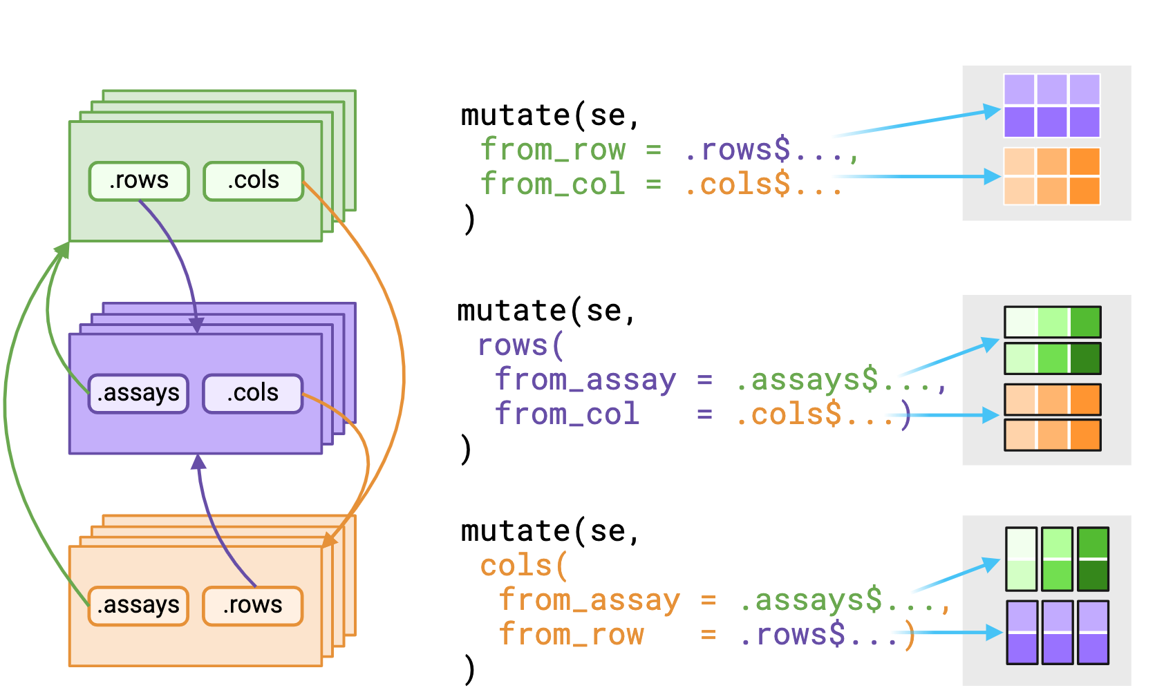
# ℹ n = 12.rows$ doing?# A SummarizedExperiment-tibble Abstraction: 3 × 2
# Groups: cols(type)
.features .samples | sum | length | type
<chr> <int> | <dbl> | <dbl> | <int>
1 A 1 | 5 | 10 | 1
2 B 1 | 7 | 20 | 1
3 C 1 | 9 | 30 | 1
4 A 2 | 17 | 10 | 2
5 B 2 | 19 | 20 | 2
6 C 2 | 21 | 30 | 2 [,1] [,2]
A 5 17
B 7 19
C 9 21xp |> # .assays_asis gives direct access to the matrix
mutate(rows(ave_counts = rowMeans(.assays_asis$counts)))# A SummarizedExperiment-tibble Abstraction: 3 × 4
.features .samples | counts | length ave_counts | type
<chr> <chr> | <int> | <dbl> <dbl> | <fct>
1 A a | 1 | 10 5.5 | 1
2 B a | 2 | 20 6.5 | 1
3 C a | 3 | 30 7.5 | 1
4 A b | 4 | 10 5.5 | 1
5 B b | 5 | 20 6.5 | 1
… … … … … … …
n-4 B c | 8 | 20 6.5 | 2
n-3 C c | 9 | 30 7.5 | 2
n-2 A d | 10 | 10 5.5 | 2
n-1 B d | 11 | 20 6.5 | 2
n C d | 12 | 30 7.5 | 2
# ℹ n = 12plyxp classA simple wrapper of SE:
plyxpFiltering, exploration, QC
Data thinning (count splitting)
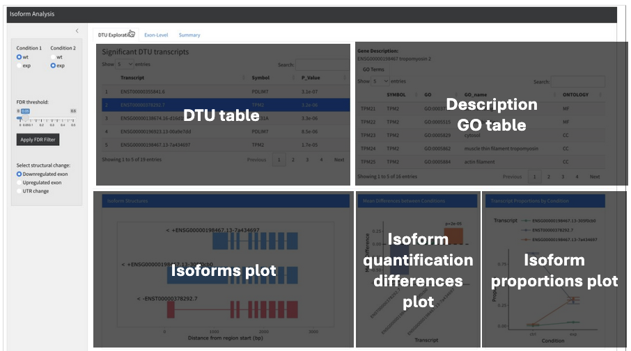
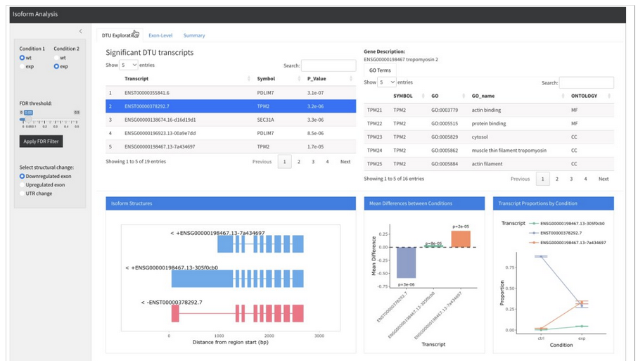
Grouping isoforms for DTU analysis, keeping track of aggregated transcript sets
Projecting splicing features from transcript-level quantification and analysis to events like skipped exons, retained introns, alternative 5’ / 3’ UTR, etc.
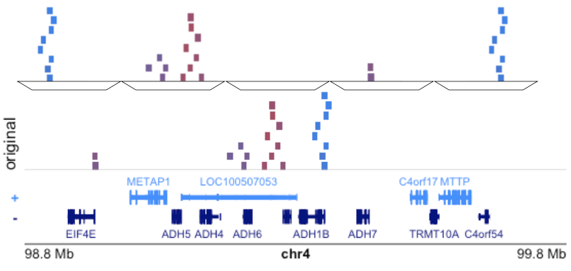
Translate biological questions about the genome into code.
Leverage familiar concepts of filters, joins, grouping, mutation, or summarization.
GRanges object with 40 ranges and 1 metadata column:
       seqnames    ranges strand |     score
          <Rle> <IRanges>  <Rle> | <numeric>
   [1]        1   114-115      * |   4.88780
   [2]        1   129-130      * |   4.40817
   [3]        1   154-155      * |   5.18773
   [4]        1   195-196      * |   5.81901
   [5]        1   200-201      * |   4.14720
   ...      ...       ...    ... .       ...
  [36]        1   898-899      * |   6.55006
  [37]        1   922-923      * |   6.46796
  [38]        1   956-957      * |   4.93079
  [39]        1   957-958      * |   4.34292
  [40]        1   966-967      * |   4.53976
  -------
seqinfo: 1 sequence from an unspecified genomeGRanges object with 30 ranges and 2 metadata columns:
seqnames ranges strand | score id
<Rle> <IRanges> <Rle> | <numeric> <factor>
[1] 1 114-115 * | 4.88780 a
[2] 1 129-130 * | 4.40817 a
[3] 1 154-155 * | 5.18773 a
[4] 1 195-196 * | 5.81901 a
[5] 1 200-201 * | 4.14720 a
... ... ... ... . ... ...
[26] 1 898-899 * | 6.55006 c
[27] 1 922-923 * | 6.46796 c
[28] 1 956-957 * | 4.93079 c
[29] 1 957-958 * | 4.34292 c
[30] 1 966-967 * | 4.53976 c
-------
seqinfo: 1 sequence from an unspecified genomex |>
filter(score > 3.5) |>
join_overlap_inner(y) |>
group_by(id) |>
summarize(ave_score = mean(score), n = n())DataFrame with 3 rows and 3 columns
id ave_score n
<factor> <numeric> <integer>
1 a 5.00465 10
2 b 5.43353 11
3 c 5.45538 7Options: directed, within, maxgap, minoverlap, etc.
GRanges object with 3 ranges and 3 metadata columns:
      seqnames    ranges strand |       id     score  distance
         <Rle> <IRanges>  <Rle> | <factor> <numeric> <integer>
  [1]        1       101      * |        a   4.88780        12
  [2]        1       451      * |        b   3.99047         1
  [3]        1       801      * |        c   6.49877        22
  -------
seqinfo: 1 sequence from an unspecified genome; no seqlengthspos_exons <- exons_flat |> filter(sign == 1)
neg_exons <- exons_flat |> filter(sign == -1)
candidates <- pos_exons |>
filter_by_non_overlaps_directed(neg_exons) |>
# ...
upstr_downreg_exons <- downreg_exons |>
flank_upstream(width = width_upstream)
seq_downreg_exons <- Hsapiens |>
getSeq(upstr_downreg_exons) |>
RNAStringSet()Asking about the enrichment of variants near genes, or peaks in TADs, often requires a lot of custom R code, lots of loops and control code.
Hard to read, hard to maintain, hard at submission/publication.
Instead: use familiar verbs, stacked genomic range sets.
We developed a package, nullranges, a modular tool to assist with making genomic comparisons.
Only provides null genomic range sets for investigating various hypotheses. That’s it!
Doesn’t do enrichment analysis per se, but can be combined with plyranges, ggplot2, etc.
Statistical papers from the ENCODE project noted that block bootstrapping genomic data preserves important spatial patterns (Bickel et al. 2010).
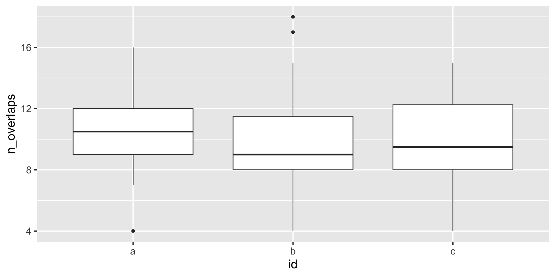
library(nullranges)
boot <- bootRanges(x, blockLength=10, R=20)
# keep track of bootstrap iteration, gives boot dist'n
boot |>
  join_overlap_inner(y) |>
  group_by(iter, id) |> # bootstrap iter, range id
  summarize(n_overlaps = n())
DataFrame with 60 rows and 3 columns
iter id n_overlaps
<Rle> <factor> <integer>
1 1 a 4
2 1 b 10
3 1 c 4
4 2 a 11
5 2 b 10
... ... ... ...
56 19 b 18
57 19 c 11
58 20 a 10
59 20 b 15
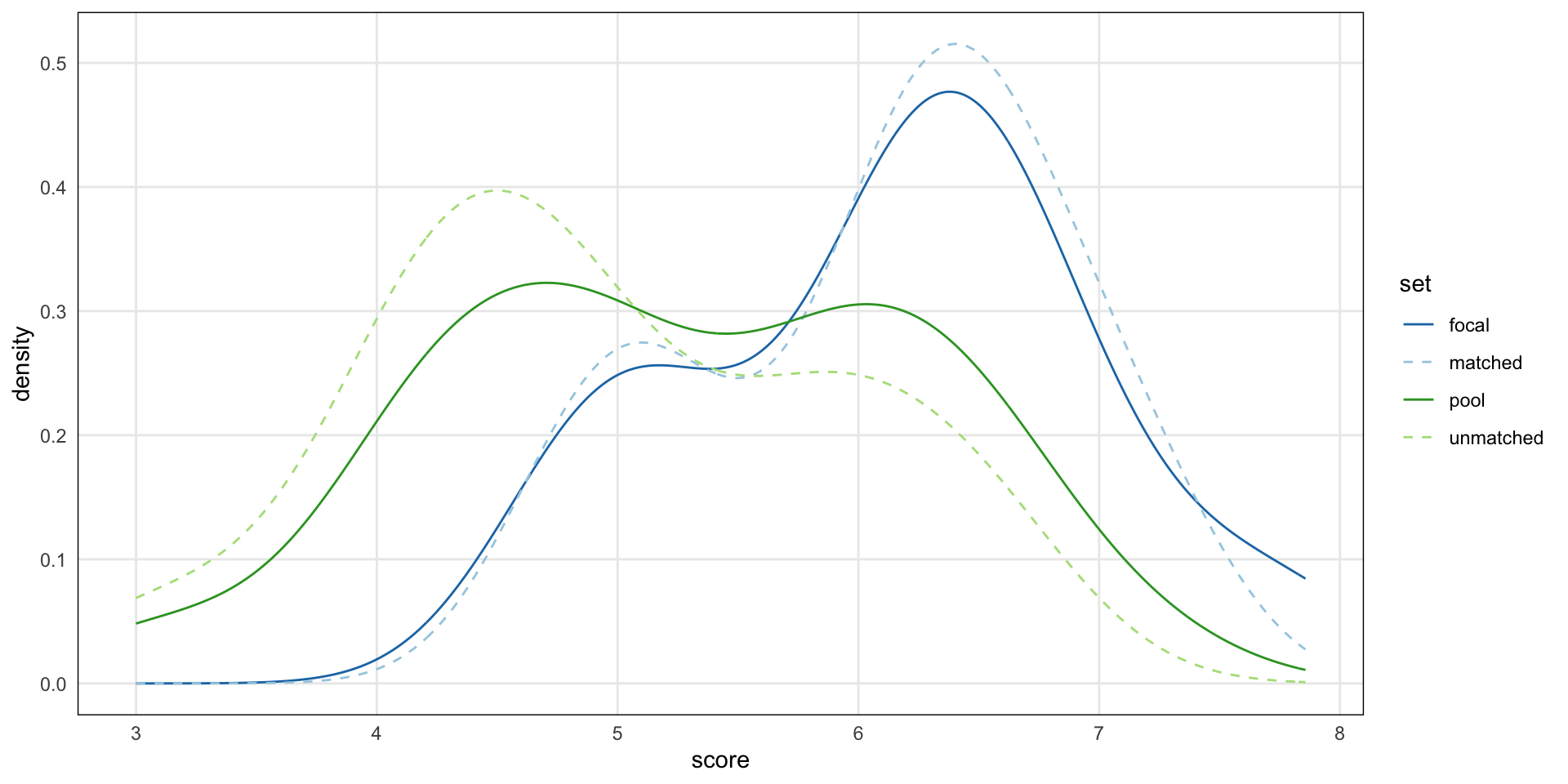
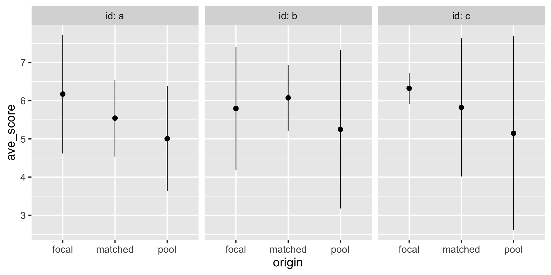
60 20 c 8Matching on covariates from a large pool allows for more focused hypothesis testing.
This is now “tidy data” with the two group concatenated and a new metadata column, origin.
DataFrame with 9 rows and 3 columns
        id  origin ave_score
  <factor>   <Rle> <numeric>
1        a   focal   6.17495
2        a matched   5.54412
3        a    pool   5.00465
4        b   focal   5.79665
5        b matched   6.07625
6        b    pool   5.25055
7        c   focal   6.32536
8        c matched   5.82463
9 c pool 5.14840Published as Application Notes in 2023:
Writing up plyxp as an Application Note.
Have shown it locally and to an industry team.
Working with Stefano Mangiola’s team on consistent printing, messaging.
Working on tutorials, workshops, documentation.
Matrix-shaped objects (SE, SCE) - Mangiola et al.
Ranges - Lee et al.
Interactions - Serizay et al.
Cytometry - Keyes et al.
Spatial - Hutchison et al.
more to come…
https://github.com/tidyomics open challenges
For project motivation, read the paper
#tidiness_in_bioc channel in Bioconductor Slack
More complicated use cases: Tidy ranges tutorial
plotPCA for bulk and OSCA for sc), also variancePartitiongeom_density of select rows/columns, or geom_violin)filter to feature, pipe to geom_point etc.)Stefano Mangiola (co-lead, tidySE, tidySCE, spatial)
Justin Landis (plyxp) and Beatriz Campillo Minano (SPLain)
Eric Davis, Wancen Mu, Doug Phanstiel (nullranges)
Stuart Lee, M. Lawrence, D. Cook (plyranges developers)
tidyomics developers: William Hutchison, Timothy Keyes, Helena Crowell, Jacques Serizay, Charlotte Soneson, Eric Davis, Noriaki Sato, Lambda Moses, Boyd Tarlinton, Abdullah Nahid, Miha Kosmac, Quentin Clayssen, Victor Yuan, Wancen Mu, Ji-Eun Park, Izabela Mamede, Min Hyung Ryu, Pierre-Paul Axisa, Paulina Paiz, Chi-Lam Poon, Ming Tang
tidyomics project funded by an Essential Open Source Software award from CZI and Wellcome Trust