The new tidy sccomp interface
Contents
![]()
![]()
![]()
We announce the new tidy and modular interface for a sccomp, which improves modularity, and clarity. The main change is the modularisation of sccomp in functions which can be linked with the pipe operator |>.
| Function | Description |
|---|---|
Estimation: sccomp_stimate() | which is usually run once in the analysis (per model). |
Testing: sccomp_test() | which candy run multiple times, depending on how many contrasts you want to test (e.g. age, untreated vs treated). |
Outlier removal: sccomp_remove_outliers() | which is usually run once after sccomp_estimate() in case you want to produce estimates not influenced by outlier data points. |
Unwanted variation removal: sccomp_remove_unwanted_variation() | which is run after sccomp_estimate() and produces a dataset that just preserve the variability of your factor of interest. |
Data replication: sccomp_replicate() | which is run after sccomp_estimate() and produces a dataset representing the theoretical data distribution according to the model (from the posterior distribution). |
Plotting: plot() | which is run after sccomp_test and outputs a series of summary plots. |
A reminder: what is sccomp
sccomp1 is a statistical model developed for differential variability analysis in compositional data, primarily used in cellular omics fields like single-cell genomics, proteomics, and microbiomics (Mangiola et al. 2023). It addresses limitations of existing methods in differential abundance analysis by incorporating several advanced features. sccomp effectively models compositional count data properties, which were previously not adequately addressed, and tackles cell-group-specific differential variability. This model uses a constrained Beta-binomial distribution to enable more precise analyses. Key capabilities of sccomp include improved differential abundance analyses through cross-sample information borrowing, outlier identification and exclusion, realistic data simulation, and facilitating cross-study knowledge transfer. By incorporating these features, sccomp provides a more comprehensive and accurate framework for analyzing cellular omics data, identifying crucial biological drivers such as disease progression markers in cancer and pathogen infection.
Installation
Bioconductor
if (!requireNamespace("BiocManager")) install.packages("BiocManager")
BiocManager::install("sccomp")
Github
devtools::install_github("stemangiola/sccomp")Deprecation of the function sccomp_glm()
The new framework
outlier_free_estimate =
  seurat_obj |>

  # Estimate
  sccomp_estimate(
    formula_composition = ~ type + continuous_covariate,
    .sample =  sample,
    .cell_group = cell_group
  ) |>

  # Remove outliers
  sccomp_remove_outliers()


# Test
outlier_free_estimate |>
  sccomp_test(contrasts = "typehealthy")
## # A tibble: 30 × 18
## cell_group parameter factor c_lower c_effect c_upper c_pH0 c_FDR c_n_eff
## <chr> <chr> <chr> <dbl> <dbl> <dbl> <dbl> <dbl> <dbl>
## 1 B immature typeheal… type 0.926 1.41 1.89 0 0 5110.
## 2 B mem typeheal… type 1.09 1.72 2.36 0 0 3857.
## 3 CD4 cm S10… typeheal… type 0.606 0.991 1.43 0 0 5290.
## 4 CD4 cm hig… typeheal… type -3.13 -1.99 -1.01 0 0 3682.
## 5 CD4 cm rib… typeheal… type -1.77 -1.06 -0.370 5.76e-3 9.18e-4 3749.
## 6 CD4 em hig… typeheal… type -2.24 -1.39 -0.603 2.50e-4 4.17e-5 3870.
## 7 CD4 naive typeheal… type 0.195 0.820 1.42 2.58e-2 5.72e-3 4786.
## 8 CD4 riboso… typeheal… type 1.53 2.04 2.53 0 0 4536.
## 9 CD8 em 1 typeheal… type -0.563 0.118 0.729 6.10e-1 1.24e-1 4336.
## 10 CD8 em 2 typeheal… type -2.12 -0.975 0.0289 6.28e-2 1.65e-2 5363.
## # ℹ 20 more rows
## # ℹ 9 more variables: c_R_k_hat <dbl>, v_lower <dbl>, v_effect <dbl>,
## # v_upper <dbl>, v_pH0 <dbl>, v_FDR <dbl>, v_n_eff <dbl>, v_R_k_hat <dbl>,
## # count_data <list>Replaces the old framework (that now will receive a deprecation warning)
  seurat_obj |>

  # Estimate
  sccomp_glm(
    formula_composition = ~ type + continuous_covariate,
    .sample =  sample,
    .cell_group = cell_group,
    check_outliers = TRUE,
    contrasts = "typehealthy"
  )
New functionalities
Removal of unwanted variation.
For visualisation purposes, we can select factor of interest we would like to preserve the effect for, end exclude all the rest. For example, if we want to produce a dataset with just the type effect, we can execute
outlier_free_estimate |>
  sccomp_remove_unwanted_variation(~ type)
## sccomp says: calculating residuals## sccomp says: regressing out unwanted factors## # A tibble: 600 × 5
## sample cell_group adjusted_proportion adjusted_counts logit_residuals
## <chr> <chr> <dbl> <dbl> <dbl>
## 1 10x_6K B immature 0.0545 255. -0.761
## 2 10x_8K B immature 0.142 1069. 0.313
## 3 GSE115189 B immature 0.112 262. 0.0162
## 4 SCP345_580 B immature 0.0890 513. -0.213
## 5 SCP345_860 B immature 0.149 958. 0.369
## 6 SCP424_pbmc1 B immature 0.111 297. -0.0372
## 7 SCP424_pbmc2 B immature 0.199 595. 0.705
## 8 SCP591 B immature 0.0244 13.9 -1.58
## 9 SI-GA-E5 B immature 0.0234 97.9 -0.737
## 10 SI-GA-E7 B immature 0.0956 702. 0.750
## # ℹ 590 more rowsPlotting
The bloating functionalities have been improved. Now, both discrete and continuous variables can be visualised overlaying the to reticle data distribution from the model. This helps the user understanding whether the model is descriptively adequate to the data.
For example, if the theoretical data distribution from the sccomp does not overlap with the observed data distribution, this is an indication that the probability distribution used by sccomp is not suitable for the data or a different model (design matrix) should be used.
outlier_free_estimate |>
  sccomp_test(contrasts = "typehealthy") |>
  plot()
## $boxplot
## $boxplot[[1]]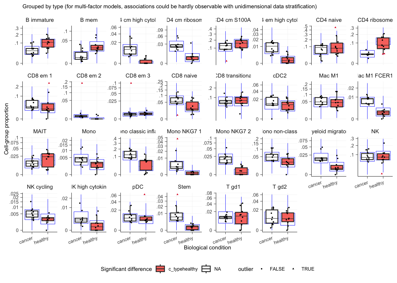
##
##
## $credible_intervals_1D
Now plotting the test against the continuous covariate
outlier_free_estimate |>
  sccomp_test(contrasts = "continuous_covariate") |>
  plot()
## $boxplot
## $boxplot[[1]]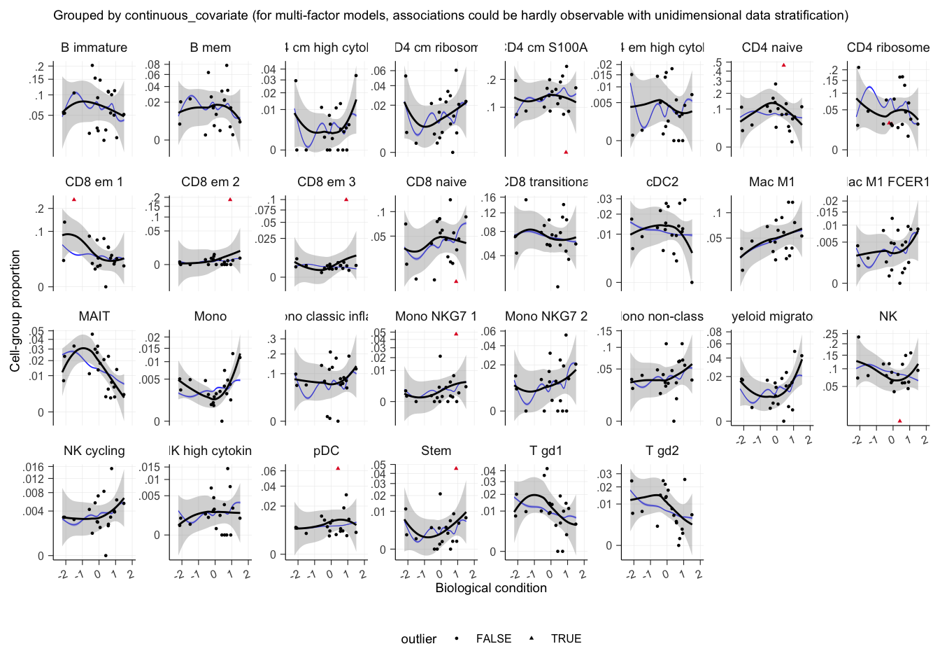
##
##
## $credible_intervals_1D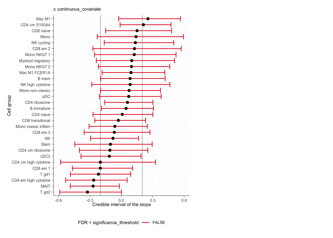
Author Stefano Mangiola
LastMod 2023-12-07