Modelling cell-type proportions in repeated-measures designs with sccomp: a TMA case study

Introduction

Cell proportions are often measured more than once in the same donor, across tumour cores or serial biopsies. The resulting observations are correlated. Averaging the cores removes ROI-level variation, while testing each phenotype separately ignores that the proportions must sum to one.

We use sccomp, a Bayesian compositional model that accepts mixed-effects designs. We fitted sccomp to a long tibble of cell counts, with one row per sample and cell type, tested the fitted model with contrasts, and predicted cell-type proportions.

Source study and study design

We apply sccomp to the NeoTRIP trial. Wang et al. (2023) used imaging mass cytometry (IMC) to map how multicellular spatial organization in triple-negative breast cancer relates to neoadjuvant immunotherapy response. In the phase III NeoTRIP trial (NCT02620280), early high-risk TNBC patients were randomised 1:1 to carboplatin + nab-paclitaxel (C) or the same regimen plus atezolizumab (C&I) for eight 3-week neoadjuvant cycles before surgery. Research FFPE biopsies:

• Baseline (n = 243)
• On-treatment (first day of cycle 2; n = 207)
• Post-treatment (surgical excision; n = 210)
• Profiled with a 43-marker IMC panel at subcellular resolution
• Deep-learning segmentation and semi-supervised clustering defined 17 epithelial and 20 TME cell phenotypes
• Multiple regions of interest (ROIs) were imaged per biopsy

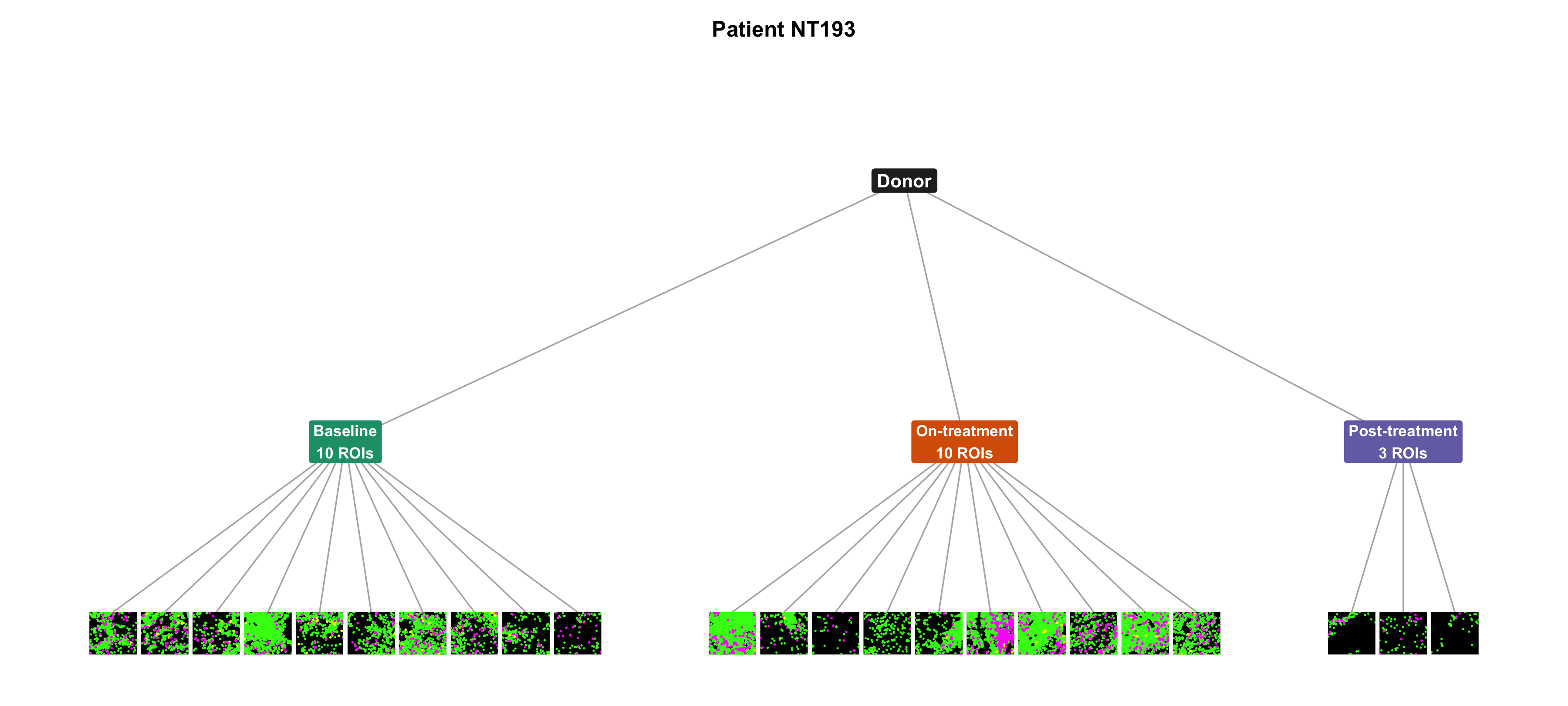
Each patient contributes several samples. The biopsies are nested in the patient, and the regions of interest are nested in the biopsy. Patient NT193, in the chemotherapy arm with residual disease, was imaged at all three timepoints: 10 ROIs at baseline, 10 on-treatment, and 3 at surgery. In the model, each ROI is one compositional sample and the patient is the repeated-measures group.

mk_spatial_tile <- function(dat, square = TRUE, pt = c(other = 0.10, pdl1 = 0.16, m2 = 0.16)) {
  if (nrow(dat) == 0) {
    dat <- tibble::tibble(
      Location_Center_X = numeric(),
      Location_Center_Y = numeric(),
      draw = character()
    )
  }
  tile <- ggplot(dat, aes(x = Location_Center_X, y = Location_Center_Y)) +
    geom_point(data = filter(dat, draw == "other"), colour = "#39FF14", size = pt[["other"]]) +
    geom_point(data = filter(dat, draw == "pdl1"), colour = "#FFFF00", size = pt[["pdl1"]]) +
    geom_point(data = filter(dat, draw == "m2"), colour = "#FF00FF", size = pt[["m2"]]) +
    scale_x_continuous(labels = NULL, guide = "none", expand = c(0, 0)) +
    scale_y_reverse(labels = NULL, guide = "none", expand = c(0, 0)) +
    theme_void(base_size = 8) +
    theme(
      plot.background = element_rect(fill = "white", colour = NA),
      panel.background = element_rect(fill = "black", colour = NA),
      legend.position = "none",
      plot.margin = margin(
        if (square) 1 else 0, if (square) 1 else 0,
        if (square) 1 else 0, if (square) 1 else 0,
        unit = "pt"
      )
    )
  if (square) tile <- tile + theme(aspect.ratio = 1)
  tile
}

roi <- read_csv(
  file.path(results_dir, "sccomp_long_tme_immune_roi.csv"),
  col_select = c(PatientID, BiopsyPhase, ImageID),
  show_col_types = FALSE
) |>
  filter(PatientID == "NT193") |>
  distinct() |>
  mutate(BiopsyPhase = factor(BiopsyPhase, phase_levels)) |>
  arrange(BiopsyPhase, ImageID) |>
  mutate(i = row_number(), .by = BiopsyPhase)

n_phase <- roi |>
  summarise(n = n(), .by = BiopsyPhase) |>
  mutate(x0 = cumsum(n + 2) - (n + 2))
roi <- roi |>
  left_join(n_phase, by = "BiopsyPhase") |>
  mutate(x = i + x0)

cells_nt <- read_fst(file.path(post_dir, "nt193-cells.fst")) |>
  as_tibble()
dx <- 0.46
pad <- 0.62
xmin <- min(roi$x) - pad
xmax <- max(roi$x) + pad
fig_w <- 12
fig_h <- 5.4
target_in <- (2 * dx) / (xmax - xmin) * fig_w
headroom <- 1.9
tile_h <- target_in * headroom / (fig_h - target_in)

phase <- roi |>
  summarise(x = mean(x), .by = BiopsyPhase) |>
  mutate(
    y = tile_h + 0.62,
    label = case_match(
      as.character(BiopsyPhase),
      "Baseline" ~ "Baseline\n10 ROIs",
      "On-treatment" ~ "On-treatment\n10 ROIs",
      "Post-treatment" ~ "Post-treatment\n3 ROIs"
    )
  )
patient <- tibble::tibble(
  x = mean(phase$x), y = phase$y[1] + 0.95, label = "Donor"
)
edges <- bind_rows(
  phase |> mutate(x, y, xend = patient$x, yend = patient$y),
  roi |> mutate(
    x,
    y = tile_h,
    xend = phase$x[match(BiopsyPhase, phase$BiopsyPhase)],
    yend = phase$y[1]
  )
)
phase_cols <- c(
  Baseline = "#1B9E77",
  `On-treatment` = "#D95F02",
  `Post-treatment` = "#7570B3"
)

tree <- ggplot() +
  geom_segment(
    data = edges, aes(x = x, y = y, xend = xend, yend = yend),
    colour = "grey70", linewidth = 0.4
  ) +
  geom_label(
    data = phase,
    aes(x, y, label = label, fill = BiopsyPhase),
    colour = "white", fontface = "bold", size = 3, label.size = 0
  ) +
  geom_label(
    data = patient, aes(x, y, label = label),
    fill = "grey15", colour = "white", fontface = "bold", size = 3.6, label.size = 0
  ) +
  scale_fill_manual(values = phase_cols, guide = "none") +
  coord_cartesian(
    xlim = c(xmin, xmax),
    ylim = c(-0.04, patient$y + 0.4),
    clip = "off"
  ) +
  labs(title = "Patient NT193") +
  theme_void(base_size = 11) +
  theme(
    plot.title = element_text(face = "bold", hjust = 0.5, size = 12),
    plot.margin = margin(6, 6, 6, 6)
  )

for (i in seq_len(nrow(roi))) {
  tree <- tree + annotation_custom(
    ggplotGrob(mk_spatial_tile(filter(cells_nt, ImageID == roi$ImageID[i]), square = FALSE)),
    xmin = roi$x[i] - dx,
    xmax = roi$x[i] + dx,
    ymin = 0,
    ymax = tile_h
  )
}
tree

Figure 1

Wang et al. linked cell densities, spatial interactions, and proliferative fractions to pathological complete response (pCR), and showed that immunotherapy remodels tissue composition over time, with response-specific dynamics of immune infiltration (notably in their Fig. 5 compositional trajectory analysis).

Quantity	Value
Per-protocol patients	257
ROI-level immune samples	1,740
Immune cell phenotypes	15
Median ROIs per patient	7

sccomp mixed-effects compositional modelling

Wang et al. summarised longitudinal composition as mean phenotype proportions per patient and compared arms, timepoints, and response groups with Wilcoxon tests, Z-scored trend plots (their Fig. 5), and per-phenotype weighted binomial GLMs on tumour-level proportions. Those tests treat each phenotype in isolation and average ROIs to the patient before inference, setting aside compositional closure (proportions sum to one) and the nesting of biopsies and ROIs within patients.

With sccomp, we model the ROI-level cell counts directly on a latent log-ratio scale with mixed effects on the mean and variability. Each ROI is one compositional sample (sample = "ROI_id" in sccomp_estimate()), several ROIs share a biopsy timepoint (BiopsyPhase), and a patient random intercept (1 | PatientID) accounts for baseline differences across individuals and shrinkage across the cohort:

\[\text{composition} \sim \text{Arm} \times \text{BiopsyPhase} \times \text{pCR} + (1 \mid \text{PatientID})\]

sccomp analysis

To retain the information from individual ROIs while accounting for repeated samples from the same patient, we analysed the immune TME compartment with each ROI as a sample and included a patient random intercept. The code can be run from top to bottom from the parsed input.

From long-format tidy input

The input long is a tibble with one row per ROI × immune phenotype: ROI_id, a count, the design columns (Arm, BiopsyPhase, pCR), and the grouping PatientID. Several ROIs share one BiopsyPhase. Preview:

library(readr)
library(dplyr)

long <- read_csv(file.path(results_dir, "sccomp_long_tme_immune_roi.csv"),
                 show_col_types = FALSE) |>
  rename(ROI_id = sample) |>
  mutate(
    count = as.integer(count),
    BiopsyPhase = factor(BiopsyPhase, c("Baseline", "On-treatment", "Post-treatment")),
    Arm = factor(Arm, c("C", "C&I")),
    pCR = factor(pCR, c("RD", "pCR"))
  )

long |>
  select(ROI_id, cell_group, count, PatientID, BiopsyPhase, Arm, pCR) |>
  gt::gt_preview() |>
  gt::tab_caption("Long-format sccomp input (1,740 ROIs x 15 immune phenotypes)")

Long-format sccomp input (1,740 ROIs x 15 immune phenotypes)

	ROI_id	cell_group	count	PatientID	BiopsyPhase	Arm	pCR
1	NTImg0011	CD8^+T	19	NT031	Baseline	C&I	RD
2	NTImg0011	CD8^+GZMB^+T	1	NT031	Baseline	C&I	RD
3	NTImg0011	CD8^+TCF1^+T	1	NT031	Baseline	C&I	RD
4	NTImg0011	CD8^+PD1^+T_{Ex}	7	NT031	Baseline	C&I	RD
5	NTImg0011	CD4^+TCF1^+T	4	NT031	Baseline	C&I	RD
6..26099
26100	NTImg1889	PD-L1^+IDO^+APCs	71	NT091	On-treatment	C&I	RD

Fit the model

To estimate response-associated changes across treatment arms and biopsy timepoints, we fitted the mixed-effects compositional model specified above.

library(sccomp)

fit <- sccomp_estimate(
  long,
  formula_composition = ~ Arm * BiopsyPhase * pCR + (1 | PatientID),
  formula_variability = ~ 1,
  sample = "ROI_id",
  cell_group = "cell_group",
  abundance = "count",
  inference_method = "hmc",
  cores = parallel::detectCores(),
  verbose = FALSE
) |>
  sccomp_test()

sccomp model
============

Model specifications:
  Family: multi_beta_binomial 
  Composition formula: ~Arm * BiopsyPhase * pCR + (1 | PatientID) 
  Variability formula: ~1 
  Inference method: hmc 

Data: Samples: 1740   Cell groups: 15 

Column prefixes: c_ -> composition parameters  v_ -> variability parameters

Convergence diagnostics:
  For each parameter, n_eff is the effective sample size and R_k_hat is the potential
  scale reduction factor on split chains (at convergence, R_k_hat = 1).

# A tibble: 4,035 × 19
   cell_group parameter  factor c_lower c_effect  c_upper   c_pH0   c_FDR c_rhat
   <chr>      <chr>      <chr>    <dbl>    <dbl>    <dbl>   <dbl>   <dbl>  <dbl>
 1 CD20^+B    (Intercep… <NA>   -0.710   -0.514  -0.314   0       0         1.00
 2 CD20^+B    ArmC&I     Arm    -0.579   -0.292  -0.00208 0.0911  3.66e-2   1.00
 3 CD20^+B    BiopsyPha… Biops… -0.0970   0.134   0.359   0.377   1.30e-1   1.00
 4 CD20^+B    BiopsyPha… Biops…  0.903    1.12    1.33    0       0         1.00
 5 CD20^+B    pCRpCR     pCR    -0.162    0.112   0.390   0.465   2.21e-1   1.00
 6 CD20^+B    ArmC&I:Bi… <NA>   -0.281    0.0545  0.396   0.602   3.17e-1   1.00
 7 CD20^+B    ArmC&I:Bi… <NA>   -0.479   -0.151   0.189   0.384   1.24e-1   1.00
 8 CD20^+B    ArmC&I:pC… <NA>   -0.227    0.164   0.540   0.368   2.55e-1   1.00
 9 CD20^+B    BiopsyPha… <NA>   -0.274    0.0505  0.377   0.625   3.86e-1   1.00
10 CD20^+B    BiopsyPha… <NA>   -0.897   -0.572  -0.259   0.00175 4.17e-4   1.00
# ℹ 4,025 more rows
# ℹ 10 more variables: c_ess_bulk <dbl>, c_ess_tail <dbl>, v_lower <dbl>,
#   v_effect <dbl>, v_upper <dbl>, v_pH0 <dbl>, v_FDR <dbl>, v_rhat <dbl>,
#   v_ess_bulk <dbl>, v_ess_tail <dbl>

We used sccomp_proportional_fold_change() to calculate how the fitted proportions changed between two conditions. We treated this as a descriptive result and used sccomp_test() for significance. Here, we compare residual disease with pathological complete response after chemoimmunotherapy at surgery:

fit |>
  sccomp_proportional_fold_change(
    formula_composition = ~ Arm * BiopsyPhase * pCR,
    from = "C&I:Post-treatment:RD",  # chemoimmunotherapy, surgery, residual disease
    to = "C&I:Post-treatment:pCR"    # same arm and visit, pathological complete response
  ) |>
  gt::gt_preview() |>
  gt::tab_caption(
    "Proportional fold change: C&I post-treatment, pCR versus residual disease"
  )

Running standalone generated quantities after 1 MCMC chain, with 1 thread(s) per chain...

Chain 1  Elapsed Time: 0.1 seconds (Generated Quantities) 
Chain 1 finished in 0.0 seconds.

Proportional fold change: C&I post-treatment, pCR versus residual disease

	cell_group	proportion_fold_change	average_uncertainty	statement
1	CD20^+B	-1.300258	0.02649652	1.3-fold decrease (from 0.0645 to 0.0496)
2	CD4^+PD1^+T	-1.595534	0.04749542	1.6-fold decrease (from 0.0439 to 0.0275)
3	CD4^+TCF1^+T	-1.100683	0.01633892	1.1-fold decrease (from 0.0918 to 0.0834)
4	CD56^+NK	1.571215	0.04918382	1.6-fold increase (from 0.0808 to 0.1269)
5	CD79a^+Plasma	1.132715	0.02740352	1.1-fold increase (from 0.0721 to 0.0816)
6..14
15	Treg	-3.406119	0.25870011	3.4-fold decrease (from 0.0275 to 0.0081)

Model checks

Convergence. To check the HMC sampling, we inspected \(\hat{R}\) and effective sample sizes. All 4,035 composition parameters have median \(\hat{R}\) = 1.001 (maximum 1.014). Bulk effective sample size has median 4,837 (minimum 495). Tail effective sample size has median 2,850 (minimum 923).

Variability is an intercept for each phenotype. Those 15 coefficients have maximum \(\hat{R}\) = 1.003, minimum bulk ESS 3,404, and minimum tail ESS 2,451. The composition parameters with the smallest bulk ESS:

fit |>
  filter(is.finite(c_ess_bulk)) |>
  slice_min(c_ess_bulk, n = 6, with_ties = FALSE) |>
  gt::gt_preview() |>
  gt::tab_caption(
    "Composition parameters with the smallest bulk effective sample size"
  )

Composition parameters with the smallest bulk effective sample size

	cell_group	parameter	factor	c_lower	c_effect	c_upper	c_pH0	c_FDR	c_rhat	c_ess_bulk	c_ess_tail	v_lower	v_effect	v_upper	v_pH0	v_FDR	v_rhat	v_ess_bulk	v_ess_tail
1	DCs	ArmC&I	Arm	-0.08375482	0.1601228	0.399447699	0.31431431	0.148577149	1.009882	600.7795	1411.607	NA	NA	NA	NA	NA	NA	NA	NA
2	DCs	(Intercept)	NA	0.77417609	0.9424418	1.116479608	0.00000000	0.000000000	1.011012	697.7882	1552.972	-3.78283	-2.957539	-2.134048	0	0	1.001649	4598.984	2582.758
3	DCs	ArmC&I:pCRpCR	NA	-0.47084651	-0.1203059	0.229162709	0.45070070	0.295827077	1.010088	717.1771	1444.238	NA	NA	NA	NA	NA	NA	NA	NA
4	M2 Mac	ArmC&I	Arm	0.12079694	0.3597968	0.601198700	0.01701702	0.009384384	1.019933	776.9721	1483.882	NA	NA	NA	NA	NA	NA	NA	NA
5	DCs	pCRpCR	pCR	-0.52733358	-0.2649256	-0.008725984	0.10010010	0.057807808	1.007276	858.1370	1509.393	NA	NA	NA	NA	NA	NA	NA	NA
6	M2 Mac	ArmC&I:pCRpCR	NA	-0.74712725	-0.4227944	-0.071407724	0.03678679	0.036786787	1.008612	878.2435	1583.149	NA	NA	NA	NA	NA	NA	NA	NA

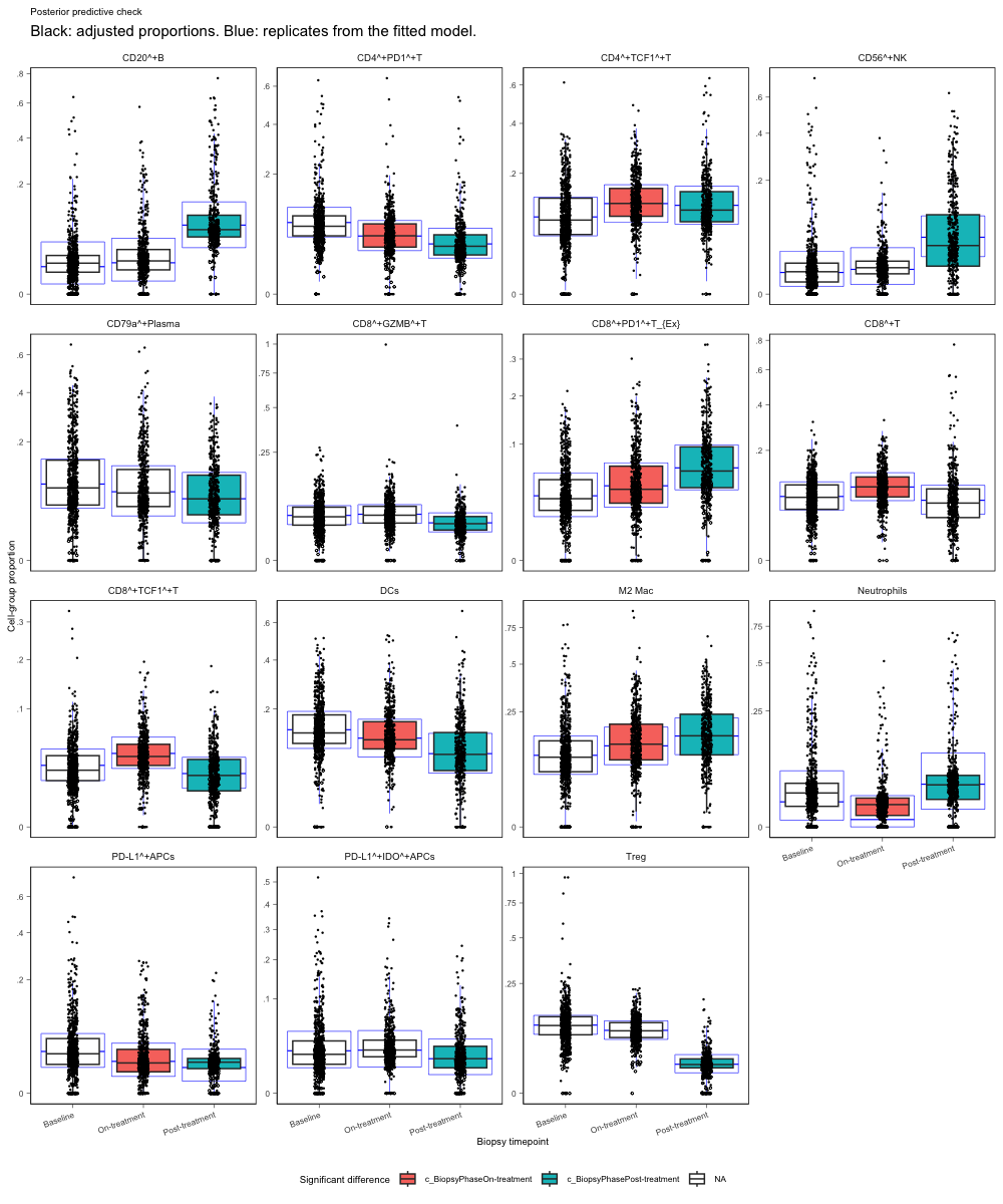
Posterior predictive check. To check whether the fitted model reproduces the observed distributions, we compared adjusted proportions with posterior predictive replicates. We set remove_unwanted_effects = TRUE to retain variation associated with biopsy timepoint. The black boxes are adjusted proportions, the blue boxes are posterior predictive replicates, and fill marks a timepoint contrast with FDR below 0.05.

fit |> 
  sccomp_boxplot(
  factor = "BiopsyPhase",
  significance_statistic = "FDR",
  remove_unwanted_effects = TRUE
  ) +
  labs(
    title = "Posterior predictive check",
    subtitle = "Black: adjusted proportions. Blue: replicates from the fitted model.",
    x = "Biopsy timepoint"
  ) +
  guides(colour = "none", shape = "none") 

Hypothesis testing

We pass contrasts to sccomp_test() as strings.

With marginal_CI_post, we compared responders with patients with residual disease at the post-treatment visit. This comparison retains any difference already present at baseline.

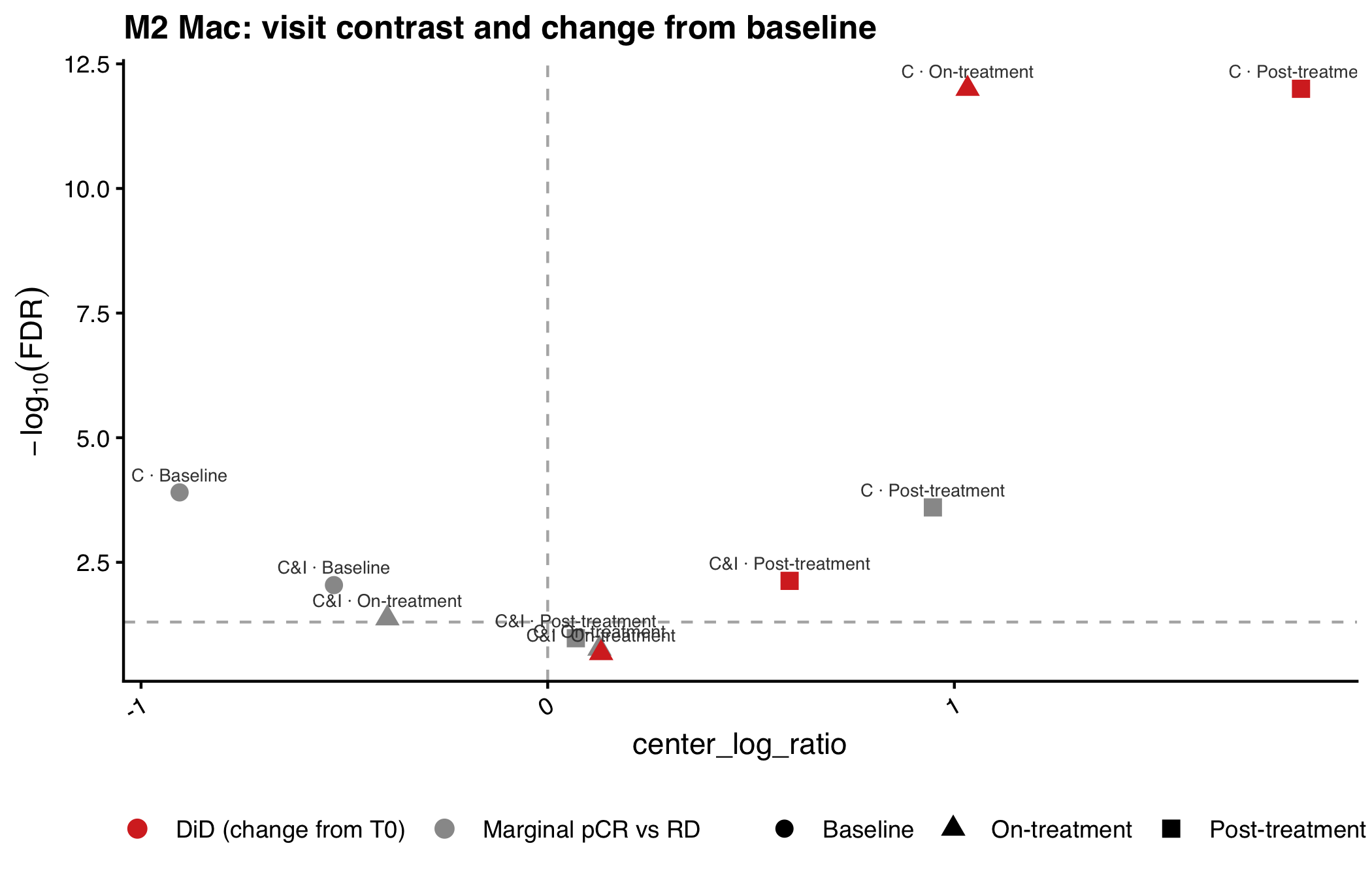
With did_CI_post, we compared their changes from baseline, thereby accounting for the difference already present at baseline. We use this contrast because a visit-only comparison retains that difference. Post-treatment M2 proportions are similar in the two response groups, so the post-treatment snapshot alone does not describe the change.

contrasts <- c(
  marginal_CI_post = paste(
    "`pCRpCR`",                                  # pCR versus RD in chemotherapy at baseline
    "`ArmC&I:pCRpCR`",                           # additional pCR versus RD gap in the C&I arm
    "`BiopsyPhasePost-treatment:pCRpCR`",        # additional pCR versus RD gap at post-treatment
    "`ArmC&I:BiopsyPhasePost-treatment:pCRpCR`", # additional pCR versus RD gap for C&I at post-treatment
    sep = " + "
  ),
  did_CI_post = paste(
    "`BiopsyPhasePost-treatment:pCRpCR`",        # change from baseline in the pCR contrast
    "`ArmC&I:BiopsyPhasePost-treatment:pCRpCR`", # further change from baseline in the C&I arm
    sep = " + "
  )
)

res <- sccomp_test(fit, contrasts = contrasts)

We stored both contrasts in res, with one row per phenotype. Below, we list the full set of difference-in-differences, strongest first:

hmc_did |>
  filter(contrast_family == "did") |>
  arrange(c_FDR) |>
  gt::gt_preview() |>
  gt::tab_caption("Change from baseline (strongest by FDR)")

Change from baseline (strongest by FDR)

	parameter	cell_group	factor	c_lower	c_effect	c_upper	c_pH0	c_FDR	c_rhat	c_ess_bulk	c_ess_tail	contrast_family	Arm	BiopsyPhase	pCR
1	did__C&I__Post_treatment	CD56^+NK	NA	2.4152900	3.25669670	4.1111366	0.0000000	0.0000000	1.0010947	4247.316	3275.396	did	C&I	Post-treatment	pCR_minus_RD
2	did__C&I__Post_treatment	DCs	NA	0.6045030	1.33237959	2.0188092	0.0000000	0.0000000	0.9996942	5122.662	3061.238	did	C&I	Post-treatment	pCR_minus_RD
3	did__C&I__Post_treatment	Neutrophils	NA	1.6664088	2.63412173	3.5857767	0.0000000	0.0000000	1.0017040	4446.958	3336.609	did	C&I	Post-treatment	pCR_minus_RD
4	did__C&I__Post_treatment	PD-L1^+APCs	NA	-3.9597930	-2.80065090	-1.6193615	0.0000000	0.0000000	1.0002327	3677.553	2867.557	did	C&I	Post-treatment	pCR_minus_RD
5	did__C&I__Post_treatment	Treg	NA	-2.8820452	-1.94723055	-1.0560065	0.0000000	0.0000000	1.0006019	2449.355	2366.402	did	C&I	Post-treatment	pCR_minus_RD
6..59
60	did__C&I__On_treatment	CD8^+TCF1^+T	NA	-0.3600534	0.01963656	0.4067838	0.6599099	0.2803971	1.0012927	5303.619	3036.666	did	C&I	On-treatment	pCR_minus_RD

Population and per-patient predictions

To visualise both the average treatment-response patterns and the variation among patients, we generated population-level and per-patient predictions.

# One row per arm, timepoint, and response group.
pop <- tibble::tribble(
  ~Arm,  ~BiopsyPhase,     ~pCR,
  "C",   "Baseline",       "RD",
  "C",   "Baseline",       "pCR",
  "C",   "On-treatment",   "RD",
  "C",   "On-treatment",   "pCR",
  "C",   "Post-treatment", "RD",
  "C",   "Post-treatment", "pCR",
  "C&I", "Baseline",       "RD",
  "C&I", "Baseline",       "pCR",
  "C&I", "On-treatment",   "RD",
  "C&I", "On-treatment",   "pCR",
  "C&I", "Post-treatment", "RD",
  "C&I", "Post-treatment", "pCR"
) |>
  mutate(
    Arm = factor(Arm, c("C", "C&I")),
    BiopsyPhase = factor(BiopsyPhase, c("Baseline", "On-treatment", "Post-treatment")),
    pCR = factor(pCR, c("RD", "pCR")),
    ROI_id = paste0("pred_", row_number()),
    PatientID = "NT031"
  )

gt::gt_preview(pop) |>
  gt::tab_caption("Population grid passed to sccomp_predict()")

Population grid passed to sccomp_predict()

	Arm	BiopsyPhase	pCR	ROI_id	PatientID
1	C	Baseline	RD	pred_1	NT031
2	C	Baseline	pCR	pred_2	NT031
3	C	On-treatment	RD	pred_3	NT031
4	C	On-treatment	pCR	pred_4	NT031
5	C	Post-treatment	RD	pred_5	NT031
6..11
12	C&I	Post-treatment	pCR	pred_12	NT031

pred_pop <- sccomp_predict(fit, new_data = pop)

Running standalone generated quantities after 1 MCMC chain, with 1 thread(s) per chain...

Chain 1  Elapsed Time: 0.185 seconds (Generated Quantities) 
Chain 1 finished in 0.0 seconds.

pred_pop |>
  gt::gt_preview() |>
  gt::tab_caption("Population predicted proportions")

Population predicted proportions

	Arm	BiopsyPhase	pCR	ROI_id	PatientID	cell_group	proportion_mean	proportion_lower	proportion_upper	unconstrained_mean	unconstrained_lower	unconstrained_upper
1	C	Baseline	RD	pred_1	NT031	CD20^+B	0.025475434	0.011849041	0.04656918	-0.78916098	-1.44397950	-0.18577897
2	C	Baseline	RD	pred_1	NT031	CD4^+PD1^+T	0.050589704	0.032262354	0.07256136	-0.07387369	-0.48652249	0.30169921
3	C	Baseline	RD	pred_1	NT031	CD4^+TCF1^+T	0.081006649	0.051677388	0.11175873	0.39988733	-0.02541777	0.76499292
4	C	Baseline	RD	pred_1	NT031	CD56^+NK	0.032822597	0.017883680	0.05537661	-0.52534173	-1.06513952	0.01087662
5	C	Baseline	RD	pred_1	NT031	CD79a^+Plasma	0.158685350	0.102258774	0.22280513	1.07227269	0.63309480	1.48362000
6..179
180	C&I	Post-treatment	pCR	pred_12	NT031	Treg	0.008723248	0.005836047	0.01223340	-1.53308238	-1.88980277	-1.19372516

# Per-patient grid: one row per patient and timepoint (uses the patient random intercept)
pat <- long |>
  distinct(PatientID, BiopsyPhase, Arm, pCR) |>
  mutate(ROI_id = paste0(PatientID, "_", BiopsyPhase))

pat |>
  gt::gt_preview() |>
  gt::tab_caption("Per-patient prediction grid (624 rows)")

Per-patient prediction grid (624 rows)

	PatientID	BiopsyPhase	Arm	pCR	ROI_id
1	NT031	Baseline	C&I	RD	NT031_Baseline
2	NT277	Baseline	C&I	RD	NT277_Baseline
3	NT277	On-treatment	C&I	RD	NT277_On-treatment
4	NT238	Baseline	C&I	RD	NT238_Baseline
5	NT238	On-treatment	C&I	RD	NT238_On-treatment
6..623
624	NT091	On-treatment	C&I	RD	NT091_On-treatment

pred_pat <- sccomp_predict(fit, new_data = pat)

Running standalone generated quantities after 1 MCMC chain, with 1 thread(s) per chain...

Chain 1  Elapsed Time: 5.094 seconds (Generated Quantities) 
Chain 1 finished in 0.0 seconds.

pred_pat

# A tibble: 9,360 × 12
   PatientID BiopsyPhase Arm   pCR   ROI_id         cell_group   proportion_mean
   <chr>     <fct>       <fct> <fct> <chr>          <chr>                  <dbl>
 1 NT031     Baseline    C&I   RD    NT031_Baseline CD20^+B               0.0175
 2 NT031     Baseline    C&I   RD    NT031_Baseline CD4^+PD1^+T           0.0427
 3 NT031     Baseline    C&I   RD    NT031_Baseline CD4^+TCF1^+T          0.0848
 4 NT031     Baseline    C&I   RD    NT031_Baseline CD56^+NK              0.0353
 5 NT031     Baseline    C&I   RD    NT031_Baseline CD79a^+Plas…          0.139 
 6 NT031     Baseline    C&I   RD    NT031_Baseline CD8^+GZMB^+T          0.0272
 7 NT031     Baseline    C&I   RD    NT031_Baseline CD8^+PD1^+T…          0.0420
 8 NT031     Baseline    C&I   RD    NT031_Baseline CD8^+T                0.0972
 9 NT031     Baseline    C&I   RD    NT031_Baseline CD8^+TCF1^+T          0.0477
10 NT031     Baseline    C&I   RD    NT031_Baseline DCs                   0.123 
# ℹ 9,350 more rows
# ℹ 5 more variables: proportion_lower <dbl>, proportion_upper <dbl>,
#   unconstrained_mean <dbl>, unconstrained_lower <dbl>,
#   unconstrained_upper <dbl>

Results

Predicted immune compositional trajectories

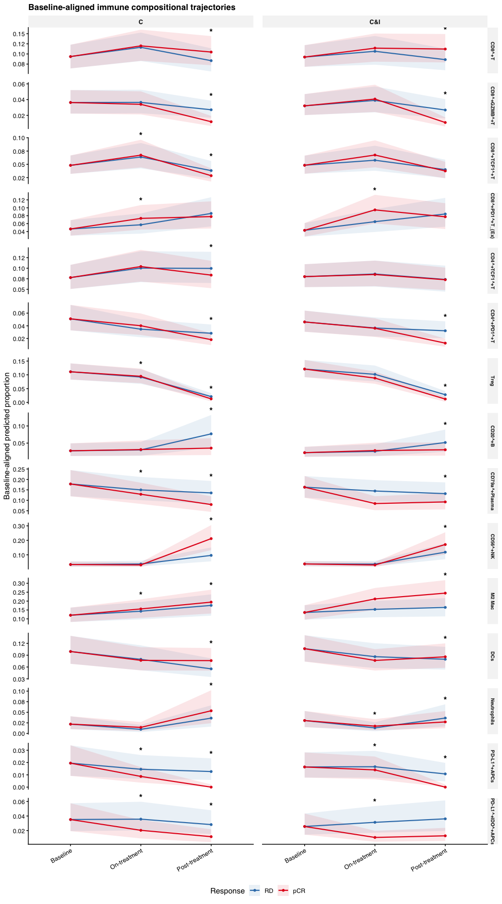
To compare the trajectories from a common starting point, we aligned both response groups to the mean of their baseline predictions for each treatment arm and cell type. We plot the predicted proportions and 95% credible intervals for all 15 immune TME phenotypes. Columns separate the treatment arms, colours separate the response groups, and asterisks mark difference-in-differences with FDR < 0.05.

# Plot shift. Within each arm and cell type, move pCR and RD to the mean of
# their baseline predictions, on the posterior draws.
draws <- sccomp_predict(
  fit, new_data = pop, number_of_draws = 500, summary_instead_of_draws = FALSE
) |>
  as_tibble() |>
  mutate(across(c(Arm, BiopsyPhase, pCR), as.character))

Running standalone generated quantities after 1 MCMC chain, with 1 thread(s) per chain...

Chain 1  Elapsed Time: 0.183 seconds (Generated Quantities) 
Chain 1 finished in 0.0 seconds.

# Shift pCR and RD to their average baseline within each Arm x cell_group, per draw
shifts <- draws |>
  filter(BiopsyPhase == "Baseline") |>
  select(Arm, cell_group, .draw, pCR, proportion) |>
  pivot_wider(names_from = pCR, values_from = proportion) |>
  mutate(shift_pCR = (pCR + RD) / 2 - pCR,
         shift_RD  = (pCR + RD) / 2 - RD) |>
  select(Arm, cell_group, .draw, shift_pCR, shift_RD)

aligned_summary <- draws |>
  left_join(shifts, by = c("Arm", "cell_group", ".draw")) |>
  mutate(aligned_prop = proportion + if_else(pCR == "pCR", shift_pCR, shift_RD)) |>
  summarise(
    aligned_mean  = mean(aligned_prop),
    aligned_lower = quantile(aligned_prop, 0.025),
    aligned_upper = quantile(aligned_prop, 0.975),
    .by = c(Arm, BiopsyPhase, pCR, cell_group)
  )

cell_order <- c(
  "CD8^+T", "CD8^+GZMB^+T", "CD8^+TCF1^+T", "CD8^+PD1^+T_{Ex}",
  "CD4^+TCF1^+T", "CD4^+PD1^+T", "Treg", "CD20^+B", "CD79a^+Plasma",
  "CD56^+NK", "M2 Mac", "DCs", "Neutrophils", "PD-L1^+APCs", "PD-L1^+IDO^+APCs"
)
cols_response <- c(RD = "#377EB8", pCR = "#E41A1C")

pred_main <- aligned_summary |>
  mutate(
    BiopsyPhase = factor(BiopsyPhase, phase_levels),
    Arm = factor(Arm, arm_levels),
    pCR = factor(pCR, c("RD", "pCR")),
    cell_group = factor(cell_group, levels = cell_order),
    # A few intervals sit just below zero after the baseline shift.
    aligned_mean = pmax(aligned_mean, 0),
    aligned_lower = pmax(aligned_lower, 0)
  )

# Asterisk just above the ribbon where the DiD FDR is below 0.05.
did_sig_fig1 <- hmc_did |>
  filter(contrast_family == "did", is.finite(c_FDR), c_FDR < 0.05) |>
  distinct(cell_group, Arm, BiopsyPhase) |>
  mutate(cell_group = factor(cell_group, levels = cell_order)) |>
  inner_join(
    pred_main |>
      summarise(ymax = max(aligned_upper), .by = c(cell_group, Arm, BiopsyPhase)),
    by = c("cell_group", "Arm", "BiopsyPhase")
  )

ggplot(pred_main, aes(x = BiopsyPhase, y = aligned_mean, colour = pCR, group = pCR)) +
  geom_ribbon(
    aes(ymin = aligned_lower, ymax = aligned_upper, fill = pCR),
    alpha = 0.10, colour = NA
  ) +
  geom_line(linewidth = 0.75) +
  geom_point(size = 1.2) +
  geom_text(
    data = did_sig_fig1,
    aes(x = BiopsyPhase, y = ymax, label = "*"),
    inherit.aes = FALSE,
    size = 4.5, colour = "black", fontface = "bold", vjust = -0.2
  ) +
  facet_grid(cell_group ~ Arm, scales = "free_y") +
  scale_y_continuous(labels = scales::label_number(accuracy = 0.01)) +
  coord_cartesian(clip = "off") +
  scale_colour_manual(values = cols_response, name = "Response") +
  scale_fill_manual(values = cols_response, name = "Response") +
  labs(
    title = "Baseline-aligned immune compositional trajectories",
    x = NULL,
    y = "Baseline-aligned predicted proportion"
  ) +
  theme_pub() +
  theme(strip.text.y = element_text(size = 7))

Figure 2

Change from baseline

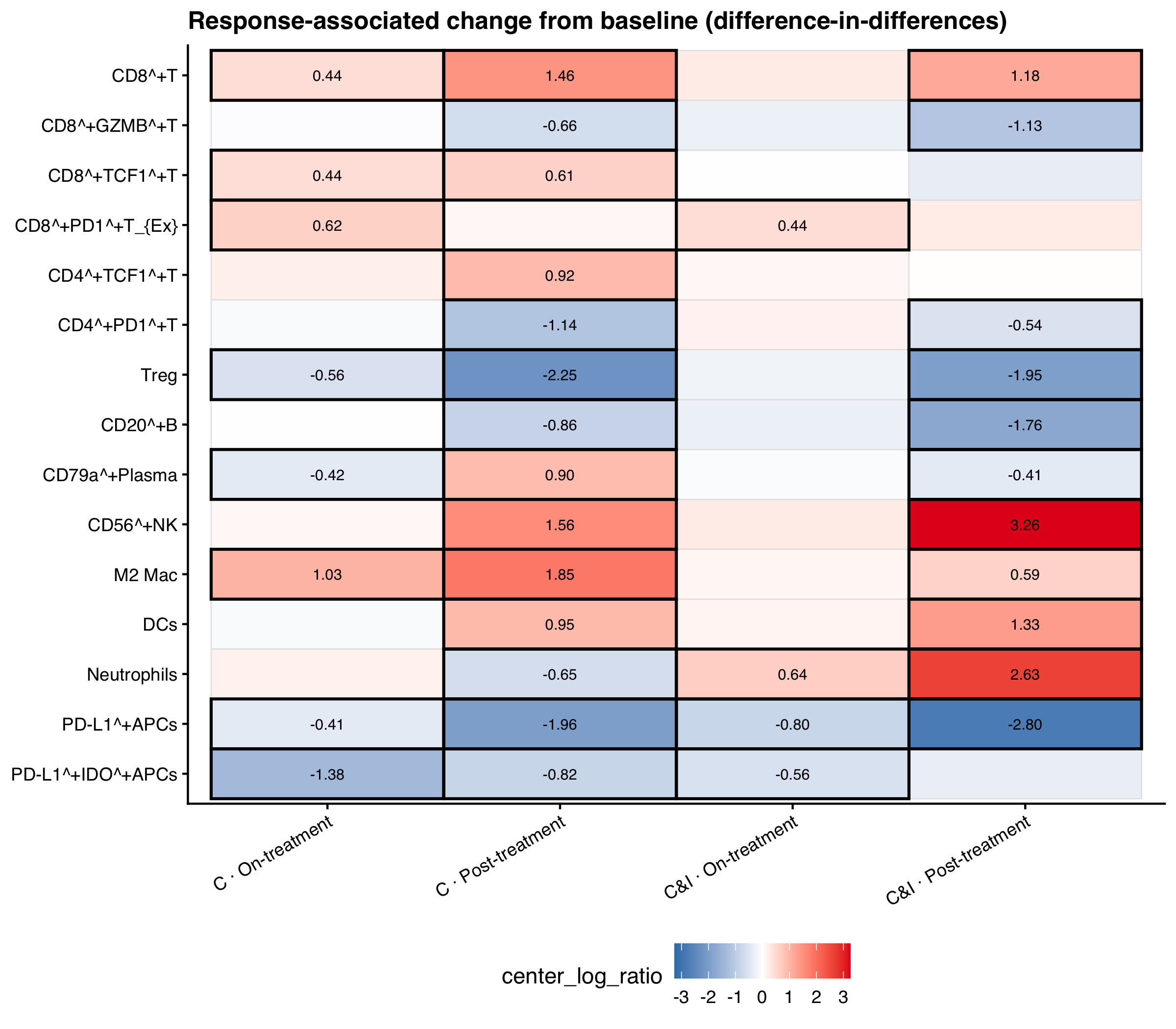
For each cell type and treatment arm, we test whether responders and patients with residual disease changed by different amounts from baseline. We plotted these contrasts for the on-treatment and post-treatment visits in Figure 2; borders mark FDR < 0.05.

did_hm <- hmc_did |>
  filter(contrast_family == "did") |>
  mutate(
    cell_group = factor(cell_group, levels = rev(cell_order)),
    BiopsyPhase = factor(BiopsyPhase, levels = c("On-treatment", "Post-treatment")),
    Arm = factor(Arm, arm_levels)
  ) |>
  filter(!is.na(cell_group)) |>
  mutate(
    sig = is.finite(c_FDR) & c_FDR < 0.05,
    facet_lab = factor(
      paste(Arm, BiopsyPhase, sep = " · "),
      levels = c(
        "C · On-treatment", "C · Post-treatment",
        "C&I · On-treatment", "C&I · Post-treatment"
      )
    )
  )

lim <- max(abs(did_hm$c_effect), na.rm = TRUE)

ggplot(did_hm, aes(x = facet_lab, y = cell_group, fill = c_effect)) +
  geom_tile(colour = "grey90", linewidth = 0.3) +
  geom_tile(
    data = filter(did_hm, sig),
    colour = "black", linewidth = 0.7, fill = NA
  ) +
  geom_text(
    aes(label = if_else(sig, sprintf("%.2f", c_effect), "")),
    size = 2.6
  ) +
  scale_fill_gradient2(
    low = cols_response[["RD"]], mid = "white", high = cols_response[["pCR"]],
    midpoint = 0, limits = c(-lim, lim), name = "Effect on\ncentered log-ratio scale"
  ) +
  labs(
    title = "Response-associated change from baseline (difference-in-differences)",
    x = NULL, y = NULL
  ) +
  theme_pub() +
  theme(
    axis.text.x = element_text(angle = 30, hjust = 1),
    panel.grid = element_blank()
  )

Figure 3

Finding: Under the difference-in-differences contrast, 14 immune phenotypes change from baseline at post-treatment, and 9 at the on-treatment visit.

Finding: In the chemoimmunotherapy arm at post-treatment, M2 macrophages increase more from baseline in patients who reach pathological complete response (FDR 0.007), while PD-L1-positive antigen-presenting cells decrease (FDR < 0.0002).

Finding: The M2 macrophage change is not detected at the on-treatment visit (FDR 0.21).

M2 macrophage changes by response

To show how the visit-specific comparison differs from the change-from-baseline analysis, we compared both M2 macrophage contrasts. Grey points compare pCR with residual disease at a single visit, whereas red points compare their changes from baseline. Points above the dotted line have FDR < 0.05.

m2_volcano <- bind_rows(
  hmc_marginal_pcr |>
    filter(cell_group == "M2 Mac") |>
    mutate(Arm, BiopsyPhase, c_effect, c_FDR, family = "Marginal pCR vs RD"),
  hmc_did |>
    filter(contrast_family == "did", cell_group == "M2 Mac") |>
    mutate(Arm, BiopsyPhase, c_effect, c_FDR, family = "DiD (change from T0)")
) |>
  mutate(label = paste(Arm, BiopsyPhase, sep = " · "))

ggplot(m2_volcano, aes(x = c_effect, y = -log10(pmax(c_FDR, 1e-12)))) +
  geom_vline(xintercept = 0, linetype = 2, colour = "grey70") +
  geom_hline(yintercept = -log10(0.05), linetype = 2, colour = "grey70") +
  geom_point(aes(colour = family, shape = BiopsyPhase), size = 2.8) +
  geom_text(aes(label = label), size = 2.3, vjust = -0.9, colour = "grey25") +
  scale_colour_manual(values = c(
    "Marginal pCR vs RD" = "#999999",
    "DiD (change from T0)" = "#d73027"
  )) +
  labs(
    title = "M2 Mac: visit contrast and change from baseline",
    x = "Effect on centered log-ratio scale",
    y = expression(-log[10](FDR)),
    colour = NULL, shape = NULL
  ) +
  theme_pub()

Figure 4

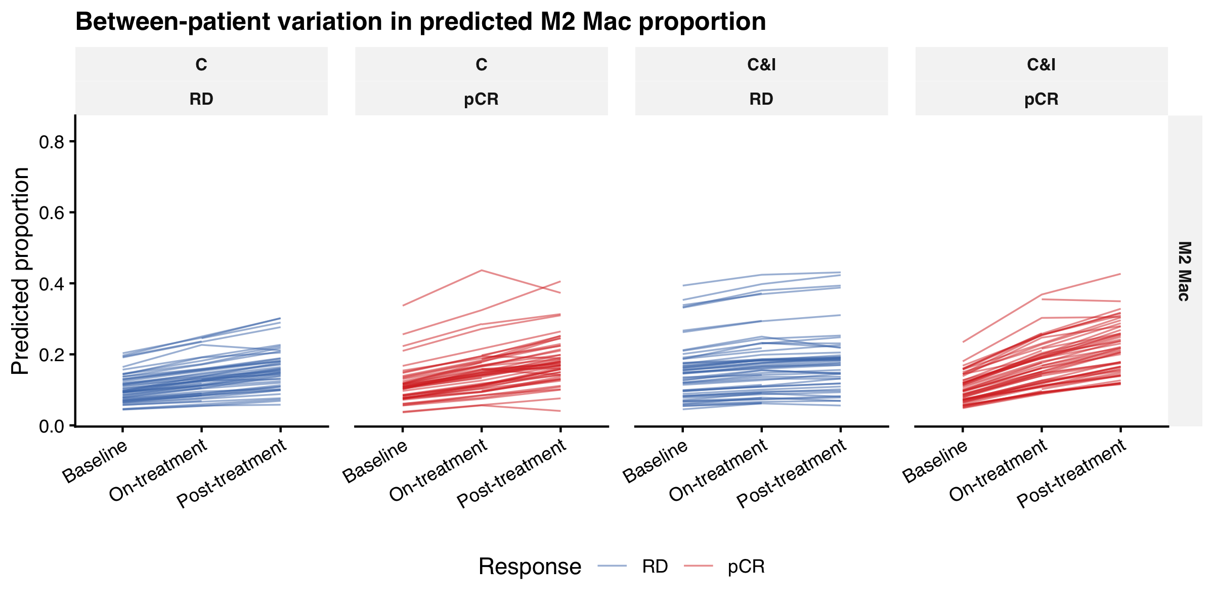
Between-patient heterogeneity in M2 Mac

To show how patients vary around the population trajectory, we estimated the population pattern using fixed effects and allowed each patient’s predictions to shift up or down using a random intercept. We did not estimate separate patient-specific slopes. We plot the resulting per-patient M2 macrophage predictions below.

pred_pat <- hmc_pred_patient |>
  filter(cell_group == "M2 Mac") |>
  mutate(cell_group = factor(cell_group))

pcr_cols <- c("RD" = "#4575b4", "pCR" = "#d73027")

ggplot(pred_pat, aes(x = BiopsyPhase, y = proportion_mean, group = PatientID, colour = pCR)) +
  geom_line(linewidth = 0.4, alpha = 0.5) +
  facet_grid(cell_group ~ Arm + pCR, scales = "free_y") +
  scale_colour_manual(values = pcr_cols, name = "Response") +
  labs(
    title = "Between-patient variation in predicted M2 Mac proportion",
    x = NULL,
    y = "Predicted proportion"
  ) +
  theme_pub() +
  theme(legend.position = "bottom", strip.text = element_text(size = 8))

Figure 5

The change on the tissue

As examples of the estimated effects, we selected four patients with paired biopsies. These examples show the direction of the contrast; the cohort estimates above give its magnitude.

Baseline regions are on the left and regions from the surgical specimen are on the right. Because they are different pieces of tissue, we compare cell-type proportions across biopsies. In these selected examples, the responders gain M2 macrophages and lose PD-L1-positive antigen-presenting cells, whereas the residual-disease patients change little. Magenta marks M2 macrophages, yellow marks PD-L1-positive antigen-presenting cells, and green marks other immune cells.

cells <- read_fst(file.path(post_dir, "did-example-cells.fst")) |> as_tibble()

examples <- tibble::tribble(
  ~PatientID, ~response, ~BiopsyPhase,       ~ImageID,    ~prop,
  "NT218",    "pCR",     "Baseline",         "NTImg1578", "M2 4.0%\nPD-L1+ APCs 12.3%",
  "NT218",    "pCR",     "Baseline",         "NTImg1579", "M2 4.0%\nPD-L1+ APCs 12.3%",
  "NT218",    "pCR",     "Baseline",         "NTImg1580", "M2 4.0%\nPD-L1+ APCs 12.3%",
  "NT218",    "pCR",     "Post-treatment",   "NTImg0491", "M2 42.4%\nPD-L1+ APCs 0.7%",
  "NT218",    "pCR",     "Post-treatment",   "NTImg0493", "M2 42.4%\nPD-L1+ APCs 0.7%",
  "NT215",    "pCR",     "Baseline",         "NTImg1181", "M2 11.1%\nPD-L1+ APCs 10.2%",
  "NT215",    "pCR",     "Baseline",         "NTImg1182", "M2 11.1%\nPD-L1+ APCs 10.2%",
  "NT215",    "pCR",     "Baseline",         "NTImg1183", "M2 11.1%\nPD-L1+ APCs 10.2%",
  "NT215",    "pCR",     "Post-treatment",   "NTImg0366", "M2 45.8%\nPD-L1+ APCs 0.4%",
  "NT215",    "pCR",     "Post-treatment",   "NTImg0372", "M2 45.8%\nPD-L1+ APCs 0.4%",
  "NT215",    "pCR",     "Post-treatment",   "NTImg0378", "M2 45.8%\nPD-L1+ APCs 0.4%",
  "NT174",    "RD",      "Baseline",         "NTImg1824", "M2 2.0%\nPD-L1+ APCs 2.1%",
  "NT174",    "RD",      "Baseline",         "NTImg1825", "M2 2.0%\nPD-L1+ APCs 2.1%",
  "NT174",    "RD",      "Baseline",         "NTImg1826", "M2 2.0%\nPD-L1+ APCs 2.1%",
  "NT174",    "RD",      "Post-treatment",   "NTImg0540", "M2 1.6%\nPD-L1+ APCs 0.8%",
  "NT174",    "RD",      "Post-treatment",   "NTImg0542", "M2 1.6%\nPD-L1+ APCs 0.8%",
  "NT028",    "RD",      "Baseline",         "NTImg1317", "M2 12.3%\nPD-L1+ APCs 1.8%",
  "NT028",    "RD",      "Baseline",         "NTImg1318", "M2 12.3%\nPD-L1+ APCs 1.8%",
  "NT028",    "RD",      "Baseline",         "NTImg1319", "M2 12.3%\nPD-L1+ APCs 1.8%",
  "NT028",    "RD",      "Post-treatment",   "NTImg0385", "M2 12.6%\nPD-L1+ APCs 1.9%",
  "NT028",    "RD",      "Post-treatment",   "NTImg0387", "M2 12.6%\nPD-L1+ APCs 1.9%"
)

tile_pt <- c(other = 0.22, pdl1 = 0.40, m2 = 0.40)

mk_note <- function(text, size = 2.7, face = "plain") {
  ggplot() +
    annotate(
      "text", x = 0.5, y = 0.5, label = text,
      fontface = face, size = size, lineheight = 0.95
    ) +
    scale_x_continuous(limits = c(0, 1), expand = c(0, 0)) +
    scale_y_continuous(limits = c(0, 1), expand = c(0, 0)) +
    theme_void()
}

mk_phase <- function(pid, phase) {
  ids <- examples |>
    filter(PatientID == pid, BiopsyPhase == phase) |>
    pull(ImageID)
  ids <- c(ids, rep(NA_character_, 3L - length(ids)))
  tiles <- lapply(ids, function(id) {
    if (is.na(id)) return(patchwork::plot_spacer())
    mk_spatial_tile(filter(cells, ImageID == id), pt = tile_pt)
  })
  prop <- examples$prop[examples$PatientID == pid & examples$BiopsyPhase == phase][1]
  patchwork::wrap_plots(
    mk_note(prop, size = 2.5),
    patchwork::wrap_plots(tiles, nrow = 1),
    ncol = 1,
    heights = c(0.22, 1)
  )
}

mk_patient <- function(pid) {
  response <- examples$response[examples$PatientID == pid][1]
  patchwork::wrap_plots(
    mk_note(paste0(pid, "\n", response), size = 3.1, face = "bold"),
    mk_phase(pid, "Baseline"),
    mk_phase(pid, "Post-treatment"),
    nrow = 1,
    widths = c(0.55, 3, 3)
  )
}

header <- patchwork::wrap_plots(
  patchwork::plot_spacer(),
  mk_note("Baseline", size = 3.4, face = "bold"),
  mk_note("Post-treatment", size = 3.4, face = "bold"),
  nrow = 1,
  widths = c(0.55, 3, 3)
)

patchwork::wrap_plots(
  header,
  mk_patient("NT218"),
  mk_patient("NT215"),
  mk_patient("NT174"),
  mk_patient("NT028"),
  ncol = 1,
  heights = c(0.28, 1, 1, 1, 1)
) +
  patchwork::plot_annotation(
    title = "Change from baseline in four chemoimmunotherapy patients",
    subtitle = "Magenta: M2 macrophages.  Yellow: PD-L1-positive APCs.  Green: other immune cells.",
    theme = theme(
      plot.title = element_text(face = "bold", size = 13),
      plot.subtitle = element_text(size = 10, colour = "grey25")
    )
  )

Figure 6

Acknowledgements

We thank Pierre-Paul Axisa (CBMR, Copenhagen, Denmark), for the helpful feedback which improved the post substantially.

---

sessionInfo()

R version 4.6.1 (2026-06-24)
Platform: aarch64-apple-darwin23
Running under: macOS Tahoe 26.6.2

Matrix products: default
BLAS:   /Library/Frameworks/R.framework/Versions/4.6/Resources/lib/libRblas.0.dylib 
LAPACK: /Library/Frameworks/R.framework/Versions/4.6/Resources/lib/libRlapack.dylib;  LAPACK version 3.12.1

locale:
[1] C.UTF-8/C.UTF-8/C.UTF-8/C/C.UTF-8/C.UTF-8

time zone: Australia/Perth
tzcode source: internal

attached base packages:
[1] stats     graphics  grDevices utils     datasets  methods   base     

other attached packages:
[1] fstcore_0.10.0  tidyr_1.3.2     dplyr_1.2.1     readr_2.2.0    
[5] patchwork_1.3.2 here_1.0.2      fst_0.9.8       ggplot2_4.0.3  

loaded via a namespace (and not attached):
 [1] tidyselect_1.2.1            farver_2.1.2               
 [3] S7_0.2.2                    fastmap_1.2.0              
 [5] SingleCellExperiment_1.34.0 tensorA_0.36.2.1           
 [7] digest_0.6.39               lifecycle_1.0.5            
 [9] sccomp_2.5.2                processx_3.9.0             
[11] magrittr_2.0.5              posterior_1.7.0            
[13] compiler_4.6.1              sass_0.4.10                
[15] rlang_1.3.0                 tools_4.6.1                
[17] gt_1.4.0                    utf8_1.2.6                 
[19] yaml_2.3.12                 data.table_1.18.4          
[21] knitr_1.51                  S4Arrays_1.12.0            
[23] labeling_0.4.3              htmlwidgets_1.6.4          
[25] bit_4.6.0                   DelayedArray_0.38.2        
[27] xml2_1.6.0                  RColorBrewer_1.1-3         
[29] cmdstanr_0.9.0              abind_1.4-8                
[31] withr_3.0.3                 purrr_1.2.2                
[33] BiocGenerics_0.58.1         grid_4.6.1                 
[35] stats4_4.6.1                scales_1.4.0               
[37] SummarizedExperiment_1.42.0 cli_3.6.6                  
[39] rmarkdown_2.31              crayon_1.5.3               
[41] generics_0.1.4              otel_0.2.0                 
[43] tzdb_0.5.0                  stringr_1.6.0              
[45] parallel_4.6.1              XVector_0.52.0             
[47] matrixStats_1.5.0           vctrs_0.7.3                
[49] Matrix_1.7-5                jsonlite_2.0.0             
[51] callr_3.8.0                 IRanges_2.46.0             
[53] hms_1.1.4                   S4Vectors_0.50.1           
[55] bit64_4.8.2                 ggrepel_0.9.8              
[57] glue_1.8.1                  ggside_0.4.1               
[59] distributional_0.8.1        stringi_1.8.7              
[61] gtable_0.3.6                GenomicRanges_1.64.0       
[63] instantiate_0.2.3           tibble_3.3.1               
[65] pillar_1.11.1               htmltools_0.5.9            
[67] Seqinfo_1.2.0               R6_2.6.1                   
[69] rprojroot_2.1.1             vroom_1.7.1                
[71] evaluate_1.0.5              Biobase_2.72.0             
[73] lattice_0.22-9              backports_1.5.1            
[75] Rcpp_1.1.2                  SparseArray_1.12.2         
[77] checkmate_2.3.4             xfun_0.60                  
[79] MatrixGenerics_1.24.0       fs_2.1.0                   
[81] forcats_1.0.1               pkgconfig_2.0.3            

© 2025 tidyomics. Content is published under Creative Commons CC-BY-4.0 License for the text and BSD 3-Clause License for any code. | R-Bloggers