Tidy genomic and transcriptomic single-cell analyses

Instructors

Dr. Stefano Mangiola is currently a Postdoctoral researcher in the laboratory of Prof. Tony Papenfuss at the Walter and Eliza Hall Institute in Melbourne, Australia. His background spans from biotechnology to bioinformatics and biostatistics. His research focuses on prostate and breast tumour microenvironment, the development of statistical models for the analysis of RNA sequencing data, and data analysis and visualisation interfaces.

Dr. Michael Love is an Associate Professor at UNC-Chapel Hill in the Department of Genetics and the Department of Biostatistics. His background is in Statistics and Computational Biology. His research is highly collaborative, working with Geneticists, Molecular Biologists, Epidemiologists, and Computer Scientists on methods for transcriptomics, epigenetics, GWAS, and high-throughput functional screens.

Workshop goals and objectives

What you will learn

Basic tidy operations possible with tidySingleCellExperiment and GRanges
How to interface SingleCellExperiment with tidy manipulation and visualisation
A real-world case study that will showcase the power of tidy single-cell methods compared with base/ad-hoc methods
Examples of how to integrate genomic and transcriptomic data (ChIP-seq and RNA-seq)

What you will not learn

The molecular technology of single-cell sequencing
The fundamentals of single-cell data analysis
The fundamentals of tidy data analysis
Detailed data integration methods (multi-view or multi-omics algorithms)

Getting started

Local

We will use the Cloud during the workshop and this method is available if you want to run the material after the workshop. If you want to install on your own computer, see instructions here.

Alternatively, you can view the material at the workshop webpage here.

Introduction slides

We provide two links to introductory material (to consult outside of the workshop slot):

Part 1 Introduction to tidySingleCellExperiment

# Load packages
library(SingleCellExperiment)
library(ggplot2)
library(plotly)
library(dplyr)
library(colorspace)
library(dittoSeq)

SingleCellExperiment is a popular data object in the Bioconductor ecosystem for representing single-cell datasets, which works seamlessly with numerous Bioconductor packages and methods written by different groups (Amezquita et al. 2020). It can easily be converted to and from other formats such as SeuratObject and scverse’s AnnData.

Here we load single-cell data in SingleCellExperiment object format. This data is peripheral blood mononuclear cells (PBMCs) from metastatic breast cancer patients.

# load single cell RNA sequencing data
sce_obj <- tidyomicsWorkshopBioc2023::sce_obj

# take a look
sce_obj

## class: SingleCellExperiment 
## dim: 482 3580 
## metadata(0):
## assays(2): counts logcounts
## rownames(482): HBB HBA2 ... TRGC2 CD8A
## rowData names(0):
## colnames(3580): 1_AAATGGACAAGTTCGT-1 1_AACAAGAGTGTTGAGG-1 ...
##   10_TTTGTTGGTACACGTT-1 10_TTTGTTGGTGATAGAT-1
## colData names(15): Barcode batch ... treatment sample
## reducedDimNames(1): UMAP
## mainExpName: SCT
## altExpNames(1): RNA

tidySingleCellExperiment provides a bridge between the SingleCellExperiment single-cell package and the tidyverse (Wickham et al. 2019). It creates an invisible layer that enables viewing the SingleCellExperiment object as a tidyverse tibble, and provides SingleCellExperiment-compatible dplyr, tidyr, ggplot and plotly functions.

For related work for bulk RNA-seq, see the tidybulk package (Mangiola et al. 2021).

If we load the tidySingleCellExperiment package and then view the single cell data, it now displays as a tibble.

library(tidySingleCellExperiment)

sce_obj

## # A SingleCellExperiment-tibble abstraction: 3,580 × 18
## # Features=482 | Cells=3580 | Assays=counts, logcounts
##    .cell       Barcode batch BCB    S.Score G2M.Score Phase cell_type nCount_RNA
##    <chr>       <fct>   <fct> <fct>    <dbl>     <dbl> <fct> <fct>          <int>
##  1 1_AAATGGAC… AAATGG… 1     BCB1… -2.07e-2   -0.0602 G1    TCR_V_De…        215
##  2 1_AACAAGAG… AACAAG… 1     BCB1…  2.09e-2   -0.0357 S     CD8+_tra…        145
##  3 1_AACGTCAG… AACGTC… 1     BCB1… -2.54e-2   -0.133  G1    CD8+_hig…        356
##  4 1_AACTTCTC… AACTTC… 1     BCB1…  2.85e-2   -0.163  S     CD8+_tra…        385
##  5 1_AAGTCGTG… AAGTCG… 1     BCB1… -2.30e-2   -0.0581 G1    MAIT             352
##  6 1_AATGAAGC… AATGAA… 1     BCB1…  1.09e-2   -0.0621 S     CD4+_rib…        335
##  7 1_ACAAAGAG… ACAAAG… 1     BCB1… -2.06e-2   -0.0409 G1    CD4+_Tcm…        242
##  8 1_ACACGCGC… ACACGC… 1     BCB1… -3.95e-4   -0.176  G1    CD8+_hig…        438
##  9 1_ACATGCAT… ACATGC… 1     BCB1… -4.09e-2   -0.0829 G1    CD4+_rib…        180
## 10 1_ACGATCAT… ACGATC… 1     BCB1…  8.82e-2   -0.0397 S     CD4+_rib…         82
## # ℹ 3,570 more rows
## # ℹ 9 more variables: nFeature_RNA <int>, nCount_SCT <int>, nFeature_SCT <int>,
## #   ident <fct>, file <chr>, treatment <chr>, sample <glue>, UMAP_1 <dbl>,
## #   UMAP_2 <dbl>

If we want to revert to the standard SingleCellExperiment view we can do that.

options("restore_SingleCellExperiment_show" = TRUE)
sce_obj

## class: SingleCellExperiment 
## dim: 482 3580 
## metadata(0):
## assays(2): counts logcounts
## rownames(482): HBB HBA2 ... TRGC2 CD8A
## rowData names(0):
## colnames(3580): 1_AAATGGACAAGTTCGT-1 1_AACAAGAGTGTTGAGG-1 ...
##   10_TTTGTTGGTACACGTT-1 10_TTTGTTGGTGATAGAT-1
## colData names(15): Barcode batch ... treatment sample

If we want to revert back to tidy SingleCellExperiment view we can.

options("restore_SingleCellExperiment_show" = FALSE)
sce_obj

## # A SingleCellExperiment-tibble abstraction: 3,580 × 18
## # Features=482 | Cells=3580 | Assays=counts, logcounts
##    .cell       Barcode batch BCB    S.Score G2M.Score Phase cell_type nCount_RNA
##    <chr>       <fct>   <fct> <fct>    <dbl>     <dbl> <fct> <fct>          <int>
##  1 1_AAATGGAC… AAATGG… 1     BCB1… -2.07e-2   -0.0602 G1    TCR_V_De…        215
##  2 1_AACAAGAG… AACAAG… 1     BCB1…  2.09e-2   -0.0357 S     CD8+_tra…        145
##  3 1_AACGTCAG… AACGTC… 1     BCB1… -2.54e-2   -0.133  G1    CD8+_hig…        356
##  4 1_AACTTCTC… AACTTC… 1     BCB1…  2.85e-2   -0.163  S     CD8+_tra…        385
##  5 1_AAGTCGTG… AAGTCG… 1     BCB1… -2.30e-2   -0.0581 G1    MAIT             352
##  6 1_AATGAAGC… AATGAA… 1     BCB1…  1.09e-2   -0.0621 S     CD4+_rib…        335
##  7 1_ACAAAGAG… ACAAAG… 1     BCB1… -2.06e-2   -0.0409 G1    CD4+_Tcm…        242
##  8 1_ACACGCGC… ACACGC… 1     BCB1… -3.95e-4   -0.176  G1    CD8+_hig…        438
##  9 1_ACATGCAT… ACATGC… 1     BCB1… -4.09e-2   -0.0829 G1    CD4+_rib…        180
## 10 1_ACGATCAT… ACGATC… 1     BCB1…  8.82e-2   -0.0397 S     CD4+_rib…         82
## # ℹ 3,570 more rows
## # ℹ 9 more variables: nFeature_RNA <int>, nCount_SCT <int>, nFeature_SCT <int>,
## #   ident <fct>, file <chr>, treatment <chr>, sample <glue>, UMAP_1 <dbl>,
## #   UMAP_2 <dbl>

It can be interacted with using SingleCellExperiment commands such as assays.

assays(sce_obj)

## List of length 2
## names(2): counts logcounts

We can also interact with our object as we do with any tidyverse tibble.

Tidyverse commands

We can use tidyverse commands, such as filter, select and mutate to explore the tidySingleCellExperiment object. Some examples are shown below and more can be seen at the tidySingleCellExperiment website here.

We can use filter to choose rows, for example, to see just the rows for the cells in G1 cell-cycle stage.

sce_obj |> filter(Phase == "G1")

## # A SingleCellExperiment-tibble abstraction: 1,859 × 18
## # Features=482 | Cells=1859 | Assays=counts, logcounts
##    .cell       Barcode batch BCB    S.Score G2M.Score Phase cell_type nCount_RNA
##    <chr>       <fct>   <fct> <fct>    <dbl>     <dbl> <fct> <fct>          <int>
##  1 1_AAATGGAC… AAATGG… 1     BCB1… -2.07e-2   -0.0602 G1    TCR_V_De…        215
##  2 1_AACGTCAG… AACGTC… 1     BCB1… -2.54e-2   -0.133  G1    CD8+_hig…        356
##  3 1_AAGTCGTG… AAGTCG… 1     BCB1… -2.30e-2   -0.0581 G1    MAIT             352
##  4 1_ACAAAGAG… ACAAAG… 1     BCB1… -2.06e-2   -0.0409 G1    CD4+_Tcm…        242
##  5 1_ACACGCGC… ACACGC… 1     BCB1… -3.95e-4   -0.176  G1    CD8+_hig…        438
##  6 1_ACATGCAT… ACATGC… 1     BCB1… -4.09e-2   -0.0829 G1    CD4+_rib…        180
##  7 1_ACGTAACG… ACGTAA… 1     BCB1… -8.69e-3   -0.140  G1    TCR_V_De…        187
##  8 1_AGAGAATT… AGAGAA… 1     BCB1… -5.14e-3   -0.102  G1    CD8+_tra…        155
##  9 1_AGATCCAT… AGATCC… 1     BCB1… -1.17e-2   -0.155  G1    CD8+_hig…        433
## 10 1_AGCCAATA… AGCCAA… 1     BCB1… -3.61e-2   -0.207  G1    CD4+_Tcm…        353
## # ℹ 1,849 more rows
## # ℹ 9 more variables: nFeature_RNA <int>, nCount_SCT <int>, nFeature_SCT <int>,
## #   ident <fct>, file <chr>, treatment <chr>, sample <glue>, UMAP_1 <dbl>,
## #   UMAP_2 <dbl>

Note that rows in this context refers to rows of the abstraction, not rows of the SingleCellExperiment which correspond to genes. tidySingleCellExperiment prioritizes cells as the units of observation in the abstraction, while the full dataset, including measurements of expression of all genes, is still available “in the background”.

We can use select to view columns, for example, to see the filename, total cellular RNA abundance and cell phase.

If we use select we will also get any view-only columns returned, such as the UMAP columns generated during the preprocessing.

sce_obj |> select(.cell, file, nCount_RNA, Phase)

## # A SingleCellExperiment-tibble abstraction: 3,580 × 6
## # Features=482 | Cells=3580 | Assays=counts, logcounts
##    .cell                file                      nCount_RNA Phase UMAP_1 UMAP_2
##    <chr>                <chr>                          <int> <fct>  <dbl>  <dbl>
##  1 1_AAATGGACAAGTTCGT-1 ../data/single_cell/SI-G…        215 G1    -3.73  -1.59 
##  2 1_AACAAGAGTGTTGAGG-1 ../data/single_cell/SI-G…        145 S      0.798 -0.151
##  3 1_AACGTCAGTCTATGAC-1 ../data/single_cell/SI-G…        356 G1    -0.292  0.515
##  4 1_AACTTCTCACGCTGAC-1 ../data/single_cell/SI-G…        385 S      0.372  2.34 
##  5 1_AAGTCGTGTGTTGCCG-1 ../data/single_cell/SI-G…        352 G1    -1.63  -0.236
##  6 1_AATGAAGCATCCAACA-1 ../data/single_cell/SI-G…        335 S      0.822  2.90 
##  7 1_ACAAAGAGTCGTACTA-1 ../data/single_cell/SI-G…        242 G1     3.28   3.97 
##  8 1_ACACGCGCAGGTACGA-1 ../data/single_cell/SI-G…        438 G1    -3.65  -0.192
##  9 1_ACATGCATCACTTTGT-1 ../data/single_cell/SI-G…        180 G1    -0.273  4.09 
## 10 1_ACGATCATCGACGAGA-1 ../data/single_cell/SI-G…         82 S     -0.816  2.90 
## # ℹ 3,570 more rows

We can use mutate to create a column. For example, we could create a new Phase_l column that contains a lower-case version of Phase.

sce_obj |>
  mutate(Phase_l = tolower(Phase)) |>
  select(.cell, Phase, Phase_l)

## # A SingleCellExperiment-tibble abstraction: 3,580 × 5
## # Features=482 | Cells=3580 | Assays=counts, logcounts
##    .cell                Phase Phase_l UMAP_1 UMAP_2
##    <chr>                <fct> <chr>    <dbl>  <dbl>
##  1 1_AAATGGACAAGTTCGT-1 G1    g1      -3.73  -1.59 
##  2 1_AACAAGAGTGTTGAGG-1 S     s        0.798 -0.151
##  3 1_AACGTCAGTCTATGAC-1 G1    g1      -0.292  0.515
##  4 1_AACTTCTCACGCTGAC-1 S     s        0.372  2.34 
##  5 1_AAGTCGTGTGTTGCCG-1 G1    g1      -1.63  -0.236
##  6 1_AATGAAGCATCCAACA-1 S     s        0.822  2.90 
##  7 1_ACAAAGAGTCGTACTA-1 G1    g1       3.28   3.97 
##  8 1_ACACGCGCAGGTACGA-1 G1    g1      -3.65  -0.192
##  9 1_ACATGCATCACTTTGT-1 G1    g1      -0.273  4.09 
## 10 1_ACGATCATCGACGAGA-1 S     s       -0.816  2.90 
## # ℹ 3,570 more rows

We can use tidyverse commands to polish an annotation column. We will extract the sample, and group information from the file name column into separate columns.

# First take a look at the file column
sce_obj |> select(.cell, file)

## # A SingleCellExperiment-tibble abstraction: 3,580 × 4
## # Features=482 | Cells=3580 | Assays=counts, logcounts
##    .cell                file                                       UMAP_1 UMAP_2
##    <chr>                <chr>                                       <dbl>  <dbl>
##  1 1_AAATGGACAAGTTCGT-1 ../data/single_cell/SI-GA-H1/outs/raw_fea… -3.73  -1.59 
##  2 1_AACAAGAGTGTTGAGG-1 ../data/single_cell/SI-GA-H1/outs/raw_fea…  0.798 -0.151
##  3 1_AACGTCAGTCTATGAC-1 ../data/single_cell/SI-GA-H1/outs/raw_fea… -0.292  0.515
##  4 1_AACTTCTCACGCTGAC-1 ../data/single_cell/SI-GA-H1/outs/raw_fea…  0.372  2.34 
##  5 1_AAGTCGTGTGTTGCCG-1 ../data/single_cell/SI-GA-H1/outs/raw_fea… -1.63  -0.236
##  6 1_AATGAAGCATCCAACA-1 ../data/single_cell/SI-GA-H1/outs/raw_fea…  0.822  2.90 
##  7 1_ACAAAGAGTCGTACTA-1 ../data/single_cell/SI-GA-H1/outs/raw_fea…  3.28   3.97 
##  8 1_ACACGCGCAGGTACGA-1 ../data/single_cell/SI-GA-H1/outs/raw_fea… -3.65  -0.192
##  9 1_ACATGCATCACTTTGT-1 ../data/single_cell/SI-GA-H1/outs/raw_fea… -0.273  4.09 
## 10 1_ACGATCATCGACGAGA-1 ../data/single_cell/SI-GA-H1/outs/raw_fea… -0.816  2.90 
## # ℹ 3,570 more rows

# Create column for sample
sce_obj <- sce_obj |>
  # Extract sample
  extract(file, "sample", "../data/.*/([a-zA-Z0-9_-]+)/outs.+", remove = FALSE)

# Take a look
sce_obj |> select(.cell, sample, everything())

## # A SingleCellExperiment-tibble abstraction: 3,580 × 18
## # Features=482 | Cells=3580 | Assays=counts, logcounts
##    .cell           sample Barcode batch BCB    S.Score G2M.Score Phase cell_type
##    <chr>           <chr>  <fct>   <fct> <fct>    <dbl>     <dbl> <fct> <fct>    
##  1 1_AAATGGACAAGT… SI-GA… AAATGG… 1     BCB1… -2.07e-2   -0.0602 G1    TCR_V_De…
##  2 1_AACAAGAGTGTT… SI-GA… AACAAG… 1     BCB1…  2.09e-2   -0.0357 S     CD8+_tra…
##  3 1_AACGTCAGTCTA… SI-GA… AACGTC… 1     BCB1… -2.54e-2   -0.133  G1    CD8+_hig…
##  4 1_AACTTCTCACGC… SI-GA… AACTTC… 1     BCB1…  2.85e-2   -0.163  S     CD8+_tra…
##  5 1_AAGTCGTGTGTT… SI-GA… AAGTCG… 1     BCB1… -2.30e-2   -0.0581 G1    MAIT     
##  6 1_AATGAAGCATCC… SI-GA… AATGAA… 1     BCB1…  1.09e-2   -0.0621 S     CD4+_rib…
##  7 1_ACAAAGAGTCGT… SI-GA… ACAAAG… 1     BCB1… -2.06e-2   -0.0409 G1    CD4+_Tcm…
##  8 1_ACACGCGCAGGT… SI-GA… ACACGC… 1     BCB1… -3.95e-4   -0.176  G1    CD8+_hig…
##  9 1_ACATGCATCACT… SI-GA… ACATGC… 1     BCB1… -4.09e-2   -0.0829 G1    CD4+_rib…
## 10 1_ACGATCATCGAC… SI-GA… ACGATC… 1     BCB1…  8.82e-2   -0.0397 S     CD4+_rib…
## # ℹ 3,570 more rows
## # ℹ 9 more variables: nCount_RNA <int>, nFeature_RNA <int>, nCount_SCT <int>,
## #   nFeature_SCT <int>, ident <fct>, file <chr>, treatment <chr>, UMAP_1 <dbl>,
## #   UMAP_2 <dbl>

We could use tidyverse unite to combine columns, for example to create a new column for sample id combining the sample and patient id (BCB) columns.

sce_obj <- sce_obj |> unite("sample_id", sample, BCB, remove = FALSE)

# Take a look
sce_obj |> select(.cell, sample_id, sample, BCB)

## # A SingleCellExperiment-tibble abstraction: 3,580 × 6
## # Features=482 | Cells=3580 | Assays=counts, logcounts
##    .cell                sample_id       sample   BCB    UMAP_1 UMAP_2
##    <chr>                <chr>           <chr>    <fct>   <dbl>  <dbl>
##  1 1_AAATGGACAAGTTCGT-1 SI-GA-H1_BCB102 SI-GA-H1 BCB102 -3.73  -1.59 
##  2 1_AACAAGAGTGTTGAGG-1 SI-GA-H1_BCB102 SI-GA-H1 BCB102  0.798 -0.151
##  3 1_AACGTCAGTCTATGAC-1 SI-GA-H1_BCB102 SI-GA-H1 BCB102 -0.292  0.515
##  4 1_AACTTCTCACGCTGAC-1 SI-GA-H1_BCB102 SI-GA-H1 BCB102  0.372  2.34 
##  5 1_AAGTCGTGTGTTGCCG-1 SI-GA-H1_BCB102 SI-GA-H1 BCB102 -1.63  -0.236
##  6 1_AATGAAGCATCCAACA-1 SI-GA-H1_BCB102 SI-GA-H1 BCB102  0.822  2.90 
##  7 1_ACAAAGAGTCGTACTA-1 SI-GA-H1_BCB102 SI-GA-H1 BCB102  3.28   3.97 
##  8 1_ACACGCGCAGGTACGA-1 SI-GA-H1_BCB102 SI-GA-H1 BCB102 -3.65  -0.192
##  9 1_ACATGCATCACTTTGT-1 SI-GA-H1_BCB102 SI-GA-H1 BCB102 -0.273  4.09 
## 10 1_ACGATCATCGACGAGA-1 SI-GA-H1_BCB102 SI-GA-H1 BCB102 -0.816  2.90 
## # ℹ 3,570 more rows

Part 2 Signature visualisation

Data pre-processing

The object sce_obj we’ve been using was created as part of a study on breast cancer systemic immune response. Peripheral blood mononuclear cells have been sequenced for RNA at the single-cell level. The steps used to generate the object are summarised below.

scran, scater, and DropletsUtils packages have been used to eliminate empty droplets and dead cells. Samples were individually quality checked and cells were filtered for good gene coverage .
Variable features were identified using modelGeneVar.
Read counts were scaled and normalised using logNormCounts from scuttle.
Data integration was performed using fastMNN with default parameters.
PCA performed to reduce feature dimensionality.
Nearest-neighbor cell networks were calculated using 30 principal components.
2 UMAP dimensions were calculated using 30 principal components.
Cells with similar transcriptome profiles were grouped into clusters using Louvain clustering from scran.

Analyse custom signature

The researcher analysing this dataset wanted to identify gamma delta T cells using a gene signature from a published paper (Pizzolato et al. 2019). We’ll show how that can be done here.

With tidySingleCellExperiment’s join_features we can view the counts for genes in the signature as columns joined to our single cell tibble.

sce_obj |>
  join_features(c("CD3D", "TRDC", "TRGC1", "TRGC2", "CD8A", "CD8B"), shape = "wide")

## # A SingleCellExperiment-tibble abstraction: 3,580 × 25
## # Features=482 | Cells=3580 | Assays=counts, logcounts
##    .cell        Barcode batch sample_id BCB    S.Score G2M.Score Phase cell_type
##    <chr>        <fct>   <fct> <chr>     <fct>    <dbl>     <dbl> <fct> <fct>    
##  1 1_AAATGGACA… AAATGG… 1     SI-GA-H1… BCB1… -2.07e-2   -0.0602 G1    TCR_V_De…
##  2 1_AACAAGAGT… AACAAG… 1     SI-GA-H1… BCB1…  2.09e-2   -0.0357 S     CD8+_tra…
##  3 1_AACGTCAGT… AACGTC… 1     SI-GA-H1… BCB1… -2.54e-2   -0.133  G1    CD8+_hig…
##  4 1_AACTTCTCA… AACTTC… 1     SI-GA-H1… BCB1…  2.85e-2   -0.163  S     CD8+_tra…
##  5 1_AAGTCGTGT… AAGTCG… 1     SI-GA-H1… BCB1… -2.30e-2   -0.0581 G1    MAIT     
##  6 1_AATGAAGCA… AATGAA… 1     SI-GA-H1… BCB1…  1.09e-2   -0.0621 S     CD4+_rib…
##  7 1_ACAAAGAGT… ACAAAG… 1     SI-GA-H1… BCB1… -2.06e-2   -0.0409 G1    CD4+_Tcm…
##  8 1_ACACGCGCA… ACACGC… 1     SI-GA-H1… BCB1… -3.95e-4   -0.176  G1    CD8+_hig…
##  9 1_ACATGCATC… ACATGC… 1     SI-GA-H1… BCB1… -4.09e-2   -0.0829 G1    CD4+_rib…
## 10 1_ACGATCATC… ACGATC… 1     SI-GA-H1… BCB1…  8.82e-2   -0.0397 S     CD4+_rib…
## # ℹ 3,570 more rows
## # ℹ 16 more variables: nCount_RNA <int>, nFeature_RNA <int>, nCount_SCT <int>,
## #   nFeature_SCT <int>, ident <fct>, file <chr>, sample <chr>, treatment <chr>,
## #   CD3D <dbl>, TRDC <dbl>, TRGC1 <dbl>, TRGC2 <dbl>, CD8A <dbl>, CD8B <dbl>,
## #   UMAP_1 <dbl>, UMAP_2 <dbl>

We can use tidyverse mutate to create a column containing the signature score. To generate the score, we scale the sum of the 4 genes, CD3D, TRDC, TRGC1, TRGC2, and subtract the scaled sum of the 2 genes, CD8A and CD8B. mutate is powerful in enabling us to perform complex arithmetic operations easily.

sce_scored <- sce_obj |>
    
  join_features(c("CD3D", "TRDC", "TRGC1", "TRGC2", "CD8A", "CD8B"), shape = "wide") |>
    
  mutate(
    signature_score =
      scales::rescale(CD3D + TRDC + TRGC1 + TRGC2, to = c(0, 1)) -
        scales::rescale(CD8A + CD8B, to = c(0, 1))
  )

sce_scored |>
  
  select(.cell, signature_score, everything())

## # A SingleCellExperiment-tibble abstraction: 3,580 × 26
## # Features=482 | Cells=3580 | Assays=counts, logcounts
##    .cell  signature_score Barcode batch sample_id BCB    S.Score G2M.Score Phase
##    <chr>            <dbl> <fct>   <fct> <chr>     <fct>    <dbl>     <dbl> <fct>
##  1 1_AAA…          0.386  AAATGG… 1     SI-GA-H1… BCB1… -2.07e-2   -0.0602 G1   
##  2 1_AAC…          0.108  AACAAG… 1     SI-GA-H1… BCB1…  2.09e-2   -0.0357 S    
##  3 1_AAC…         -0.789  AACGTC… 1     SI-GA-H1… BCB1… -2.54e-2   -0.133  G1   
##  4 1_AAC…         -0.0694 AACTTC… 1     SI-GA-H1… BCB1…  2.85e-2   -0.163  S    
##  5 1_AAG…          0      AAGTCG… 1     SI-GA-H1… BCB1… -2.30e-2   -0.0581 G1   
##  6 1_AAT…          0      AATGAA… 1     SI-GA-H1… BCB1…  1.09e-2   -0.0621 S    
##  7 1_ACA…          0.108  ACAAAG… 1     SI-GA-H1… BCB1… -2.06e-2   -0.0409 G1   
##  8 1_ACA…          0.170  ACACGC… 1     SI-GA-H1… BCB1… -3.95e-4   -0.176  G1   
##  9 1_ACA…          0      ACATGC… 1     SI-GA-H1… BCB1… -4.09e-2   -0.0829 G1   
## 10 1_ACG…          0.278  ACGATC… 1     SI-GA-H1… BCB1…  8.82e-2   -0.0397 S    
## # ℹ 3,570 more rows
## # ℹ 17 more variables: cell_type <fct>, nCount_RNA <int>, nFeature_RNA <int>,
## #   nCount_SCT <int>, nFeature_SCT <int>, ident <fct>, file <chr>,
## #   sample <chr>, treatment <chr>, CD3D <dbl>, TRDC <dbl>, TRGC1 <dbl>,
## #   TRGC2 <dbl>, CD8A <dbl>, CD8B <dbl>, UMAP_1 <dbl>, UMAP_2 <dbl>

The gamma delta T cells could then be visualised by the signature score using Bioconductor’s visualisation functions.

sce_scored |>
    
  scater::plotUMAP(colour_by = "signature_score")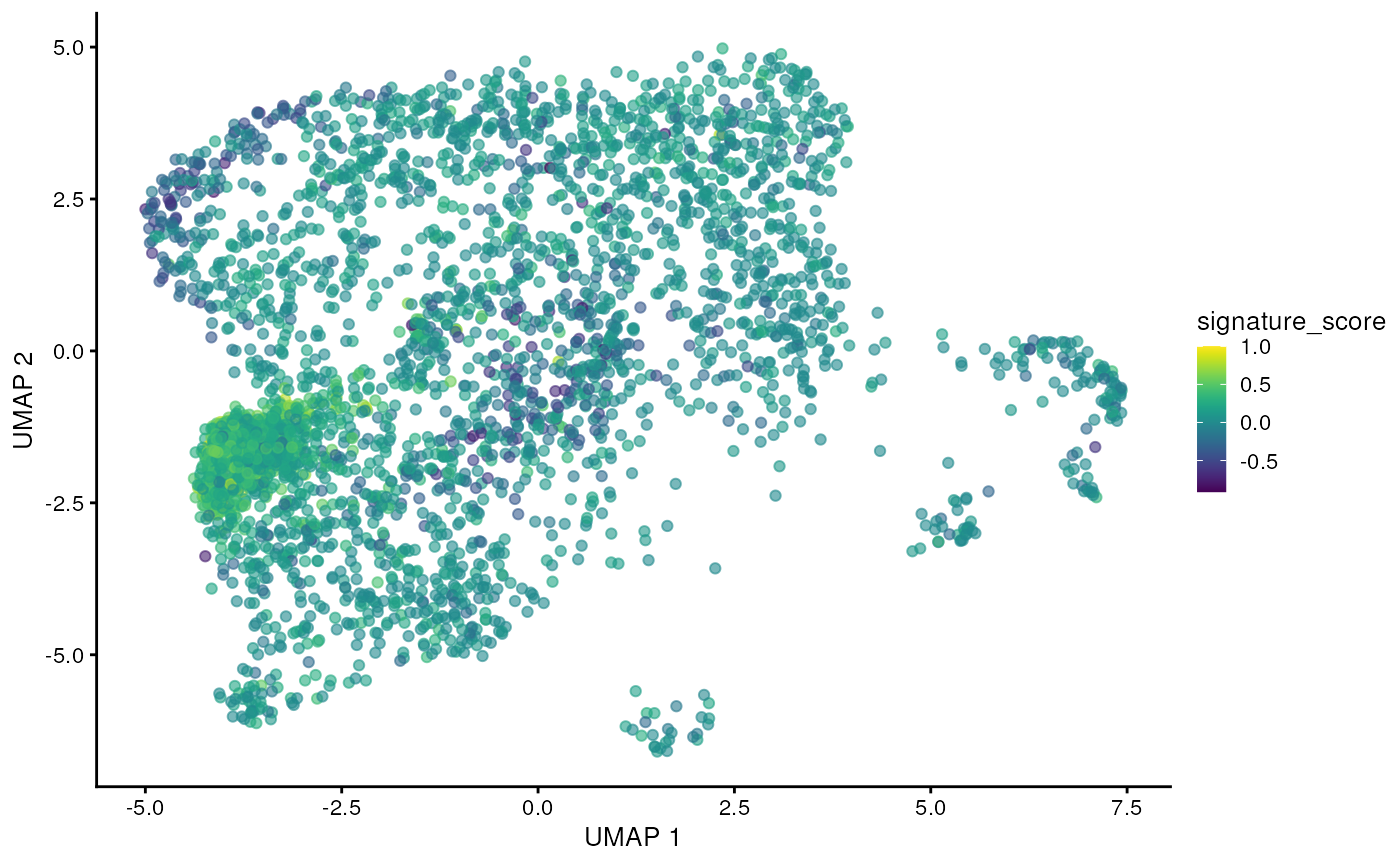

The cells could also be visualised using the popular and powerful ggplot2 package, enabling the researcher to use ggplot functions they were familiar with, and to customise the plot with great flexibility.

sce_scored |>
    
  # plot cells with high score last so they're not obscured by other cells
  arrange(signature_score) |>
    
  ggplot(aes(UMAP_1, UMAP_2, color = signature_score)) +
  geom_point() +
  scale_color_distiller(palette = "Spectral") +
  tidyomicsWorkshopBioc2023::theme_multipanel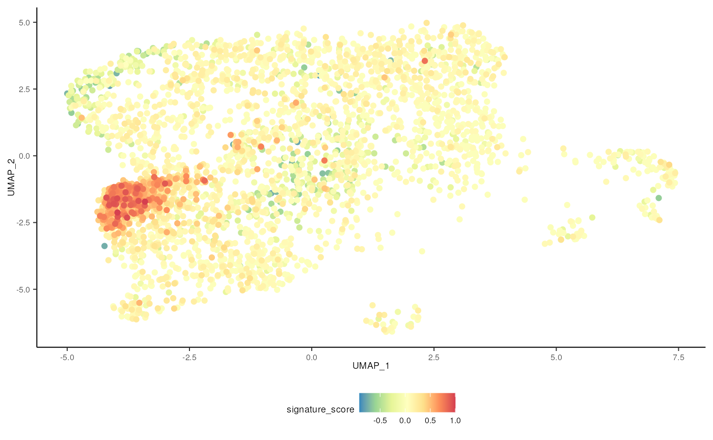

For exploratory analyses, we can select the gamma delta T cells, the red cluster on the left with high signature score. We’ll filter for cells with a signature score > 0.7.

sce_obj_gamma_delta <-
    
  sce_scored |>
    
    # Proper cluster selection should be used instead (see supplementary material)
  filter(signature_score > 0.7)

For comparison, we show the alternative using base R and SingleCellExperiment. Note that the code contains more redundancy and intermediate objects.

counts_positive <-
  assay(sce_obj, "logcounts")[c("CD3D", "TRDC", "TRGC1", "TRGC2"), ] |>
  colSums() |>
  scales::rescale(to = c(0, 1))

counts_negative <-
  assay(sce_obj, "logcounts")[c("CD8A", "CD8B"), ] |>
  colSums() |>
  scales::rescale(to = c(0, 1))

sce_obj$signature_score <- counts_positive - counts_negative

sce_obj_gamma_delta <- sce_obj[, sce_obj$signature_score > 0.7]

We can then focus on just these gamma delta T cells and chain Bioconductor and tidyverse commands together to analyse.

library(batchelor)
library(scater)

sce_obj_gamma_delta <-
    
  sce_obj_gamma_delta |>
    
  # Integrate - using batchelor.
  multiBatchNorm(batch = colData(sce_obj_gamma_delta)$sample) |>
  fastMNN(batch = colData(sce_obj_gamma_delta)$sample) |>
    
  # Join metadata removed by fastMNN - using tidyverse
  left_join(as_tibble(sce_obj_gamma_delta)) |>
    
  # Dimension reduction - using scater
  runUMAP(ncomponents = 2, dimred = "corrected")

Visualise gamma delta T cells. As we have used rough threshold we are left with only few cells. Proper cluster selection should be used instead (see supplementary material).

sce_obj_gamma_delta |> plotUMAP()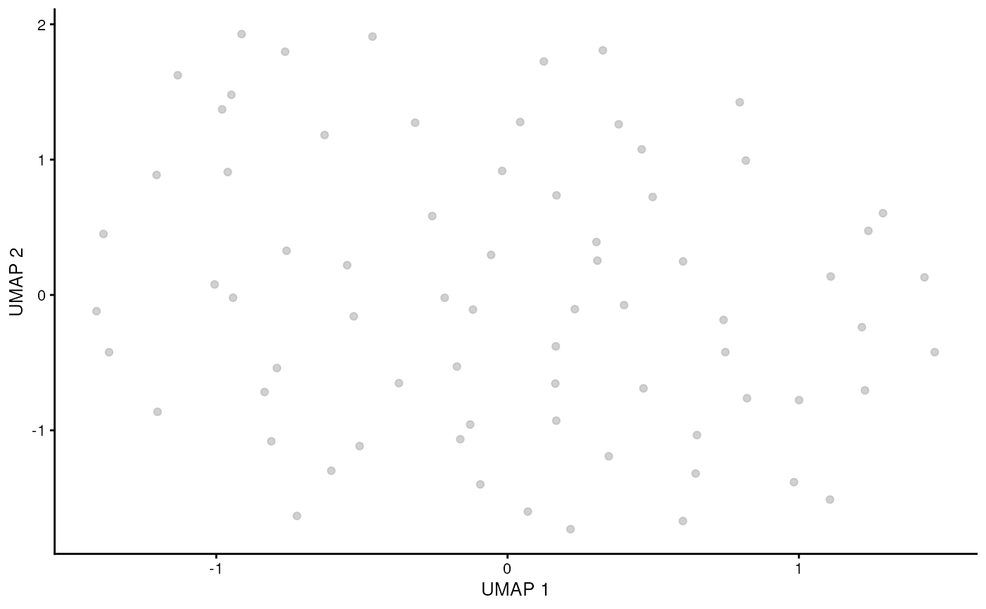

It is also possible to visualise the cells as a 3D plot using plotly. The example data used here only contains a few genes, for the sake of time and size in this demonstration, but below is how you could generate the 3 dimensions needed for 3D plot with a full dataset.

single_cell_object |>
  RunUMAP(dims = 1:30, n.components = 3L, spread = 0.5, min.dist = 0.01, n.neighbors = 10L)

We’ll demonstrate creating a 3D plot using some data that has 3 UMAP dimensions. This is a fantastic way to visualise both reduced dimensions and metadata in the same representation.

pbmc <- tidyomicsWorkshopBioc2023::sce_obj_UMAP3

pbmc |>
  plot_ly(
    x = ~`UMAP_1`,
    y = ~`UMAP_2`,
    z = ~`UMAP_3`,
    color = ~cell_type,
    colors = dittoSeq::dittoColors()
  ) %>%
  add_markers(size = I(1))

Exercises

Using the sce_obj:

What proportion of all cells are gamma-delta T cells? Use signature_score > 0.7 to identify gamma-delta T cells.
There is a cluster of cells characterised by a low RNA output (nCount_RNA < 100). Identify the cell composition (cell_type) of that cluster.

Part 3 Genomic and transcriptomic data integration

So far we have examined expression of genes across our cells, but we haven’t considered the genomic location of the genes. In this section we will operate on genomic location information using the plyranges (Stuart Lee, Cook, and Lawrence 2019) package, and tie this to the single cell transcriptomics data we have been examining.

plyranges provides tidyverse-style functionality to genomic ranges (GRanges objects (Lawrence et al. 2013)) analogous to how tidySingleCellExperiment provides functionality for SingleCellExperiment objects. For an example of a workflow using plyranges as part of a bulk RNA-seq analysis, see S. Lee, Lawrence, and Love (2020).

In some pipelines (e.g. using tximeta (Love 2020) to import bulk or single-cell quantification data) our SingleCellExperiment or SummarizedExperiment would already have genomic range information attached to the rows of the object. That is, we would have information about the starts and ends of the genes, their strand information, even the lengths of the chromosomes and the genome build, etc.

Before we start our integrative analysis, we will first take some steps to add hg38 range information on our genes, matching by the gene symbol provided on the rows of sce_obj. We add genes from the ensembldb package (Rainer, Gatto, and Weichenberger 2019) (to see how to add a particular version of Ensembl, see the package vignette).

# what our rownames look like: gene symbols
sce_obj |> rownames() |> head()

## [1] "HBB"    "HBA2"   "HBA1"   "S100A9" "LYZ"    "S100A8"

# we recommend Ensembl or GENCODE gene annotations
edb <- EnsDb.Hsapiens.v86::EnsDb.Hsapiens.v86 # hg38
g <- ensembldb::genes(edb)
head(genome(g))

##        1       10       11       12       13       14 
## "GRCh38" "GRCh38" "GRCh38" "GRCh38" "GRCh38" "GRCh38"

We can examine the first three genes and their metadata:

library(plyranges)
g |> slice(1:3)

## GRanges object with 3 ranges and 6 metadata columns:
##                   seqnames      ranges strand |         gene_id   gene_name
##                      <Rle>   <IRanges>  <Rle> |     <character> <character>
##   ENSG00000223972        1 11869-14409      + | ENSG00000223972     DDX11L1
##   ENSG00000227232        1 14404-29570      - | ENSG00000227232      WASH7P
##   ENSG00000278267        1 17369-17436      - | ENSG00000278267   MIR6859-1
##                             gene_biotype seq_coord_system      symbol
##                              <character>      <character> <character>
##   ENSG00000223972 transcribed_unproces..       chromosome     DDX11L1
##   ENSG00000227232 unprocessed_pseudogene       chromosome      WASH7P
##   ENSG00000278267                  miRNA       chromosome   MIR6859-1
##                                         entrezid
##                                           <list>
##   ENSG00000223972 100287596,100287102,727856,...
##   ENSG00000227232                           <NA>
##   ENSG00000278267                      102466751
##   -------
##   seqinfo: 357 sequences (1 circular) from GRCh38 genome

Our first task is to subset g, the human genes, to the ones in our SingleCellExperiment. While Ensembl IDs are unique, gene symbols are not, so we will have to also remove any duplicate gene symbols (recommend working with Ensembl IDs as feature identifiers when possible).

We subset the columns of g to just the symbol column, using the select() function. plyranges enables us to use familiar tidy verbs on GRanges objects, e.g. to filter rows or to select columns of metadata attached to the ranges.

g <- g |>

  select(symbol)

g |> slice(1:3)

## GRanges object with 3 ranges and 1 metadata column:
##                   seqnames      ranges strand |      symbol
##                      <Rle>   <IRanges>  <Rle> | <character>
##   ENSG00000223972        1 11869-14409      + |     DDX11L1
##   ENSG00000227232        1 14404-29570      - |      WASH7P
##   ENSG00000278267        1 17369-17436      - |   MIR6859-1
##   -------
##   seqinfo: 357 sequences (1 circular) from GRCh38 genome

Now we filter the genes of our SingleCellExperiment to only those present as rownames of sce_obj, and remove duplicate IDs. We then sort by genomic location, and use the gene symbols as names of the ranges.

gene_names <- sce_obj |> rownames()

g <- g |>
  
  filter(symbol %in% gene_names) |>
  filter(!duplicated(symbol)) |>
  sort() # genomic position sorting

names(g) <- g$symbol

Now we can add our gene information to the rows of the sce_obj.

Again, these following steps would not be necessary using a pipeline that imports quantification data to ranged objects, but it isn’t too hard to add manually. If adding ranges manually, make note of the provenance of where you downloaded the information (Ensembl, GENCODE or otherwise), and assign a genome build if you plan on sharing the final object (e.g. with genome(x) <- "...").

all(names(g) %in% rownames(sce_obj))

## [1] TRUE

sce_sub <- sce_obj[ names(g), ] # put SCE in order of `g`
rowRanges(sce_sub) <- g # assign ranges `g` to the SCE
sce_sub |> rowRanges() # peek at the ranges

## GRanges object with 447 ranges and 1 metadata column:
##              seqnames              ranges strand |      symbol
##                 <Rle>           <IRanges>  <Rle> | <character>
##        ISG15        1     1001138-1014541      + |       ISG15
##         C1QA        1   22636506-22639608      + |        C1QA
##         C1QB        1   22652762-22661538      + |        C1QB
##   ZNF436-AS1        1   23368997-23371839      + |  ZNF436-AS1
##        RCAN3        1   24502351-24541040      + |       RCAN3
##          ...      ...                 ...    ... .         ...
##        ALAS2        X   55009055-55031064      - |       ALAS2
##       NAP1L3        X   93670930-93673568      - |      NAP1L3
##     TMEM255A        X 120258650-120311556      - |    TMEM255A
##      SMARCA1        X 129446501-129523500      - |     SMARCA1
##         MPP1        X 154778684-154821007      - |        MPP1
##   -------
##   seqinfo: 357 sequences (1 circular) from GRCh38 genome

Now let’s do something interesting with the gene ranges: let’s see if genes near peaks of active chromatin marks (H3K4me3 measured with ChIP-seq) in another experiment involving PBMC have a difference in their expression level compared to other genes.

There are many sources of epigenetic tracks, ENCODE, Roadmap, etc. Here we will use some ENCODE (ENCODE 2012) data available in AnnotationHub on Bioconductor.

We had to do a bit of book-keeping first. These peaks were in the hg19 genome build, so we have ran the following commands (here un-evaluated) to ’lift” the peaks to the hg38 genome build, and provide proper sequence information.

### un-evaluated code chunk ###
# AnnotationHub contains many useful genome tracks
library(AnnotationHub)
ah <- AnnotationHub()
# can be queried with keywords
query(ah, c("Peripheral_Blood","h3k4me3"))
# downloading a particular resource
peaks <- ah[["AH44823"]]
library(rtracklayer)
# lifting hg19 to hg38
new_peaks <- unlist(
  liftOver(
    peaks,
    chain = import.chain("~/Downloads/hg19ToHg38.over.chain")
  )
)
# Ensembl-style chrom names
seqlevelsStyle(new_peaks) <- "NCBI"
# bring over any missing chroms
seqlevels(new_peaks) <- seqlevels(sce_sub)
# bring over chrom lengths
seqinfo(new_peaks) <- seqinfo(sce_sub)
# subset to a few columns
pbmc_h3k4me3_hg38 <- new_peaks |>
  select(signalValue, qValue, peak)
# save for reloading below
save(pbmc_h3k4me3_hg38, file="data/pbmc_h3k4me3_hg38.rda", compress="xz")

Loading those peaks.

# loading those H3K4me3 peaks for PBMCs
peaks <- tidyomicsWorkshopBioc2023::pbmc_h3k4me3_hg38
plot(peaks$qValue, type="l", ylab="q-value", main="H3K4me3 peaks")
abline(v=5000, lty=2)

We will arbitrarily chose to take the top 5,000 peaks by p-value. How to chose the number of epigenetic peaks and genes to consider in a multi-omics analysis is a more involved question, and is worth considering the impact of such a choice for enrichment analysis.

peaks <- peaks |>
  
  slice(1:5000) |> # ordered already by p-value (most to least sig)
  sort() # genomic position sorting

It is easy to compute the distance of the genes in our SingleCellExperiment to the nearest H3K4me3 peak, using plyranges convenience functions.

See the plyranges package website for a full listing of such functions.

dists <- rowRanges(sce_sub) |>

  anchor_5p() |> # anchor 5 prime end
  mutate(width=1) |> # shrink range to 1bp
  add_nearest_distance(peaks)

hist(log10(dists$distance + 1), breaks=40,
     main="gene-to-peak distance", xlab="log10 distance")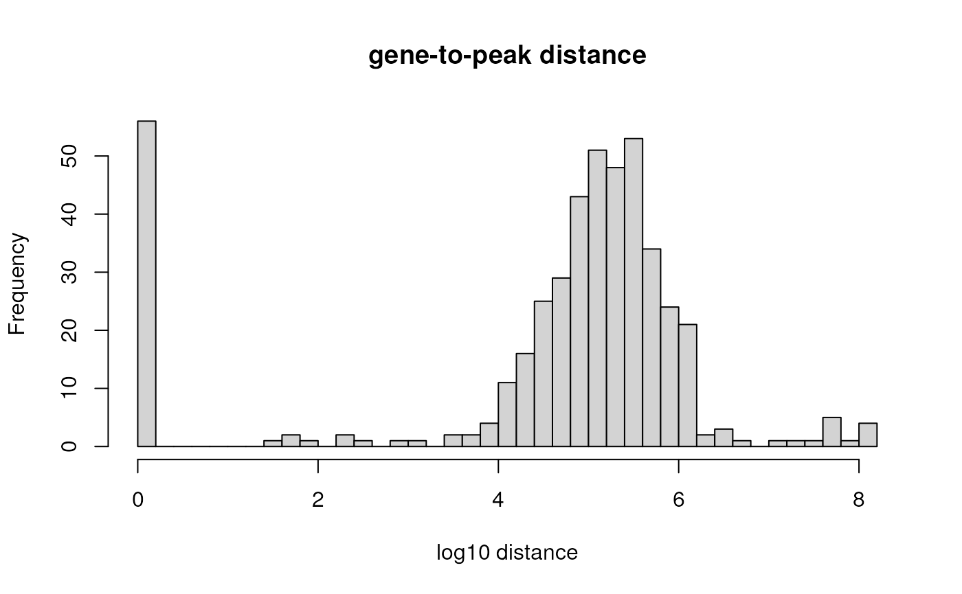

Let’s put the genes into 4 different bins by their distance to a H3K4me3 peak: 1) overlapping [distance of 0], 2) 1bp-10kb, 3) 10kb-100kb, or 4) farther than 100kb.

bins <- c(0,1,1e4,1e5,Inf)

dists <- dists |>
  
  select(symbol, distance, .drop_ranges = TRUE) |> # remove chr/pos/strand etc.
  as_tibble() |>
  mutate(distance_bin = cut(distance, bins, include.lowest = TRUE)) |>
  rename(feature = symbol) # this will help us add information to the SCE

We can see how many genes are in which category:

dists |>
  
  ggplot(aes(distance_bin)) +
  geom_bar()

We will now take the SingleCellExperiment data and compress it down to a SummarizedExperiment using the aggregate_cells function from tidySingleCellExperiment. After this function, every column of the SummarizedExperiment is a cell type.

We immediately pipe the SummarizedExperiment into a left_join where we add the distance-to-peak information, and then into a nest command where we create a nested (tidy)SummarizedExperiment object, where we have grouped by the distance bin that the genes fall into.

library(tidySummarizedExperiment)
library(purrr)
nested <- sce_sub |>
  
  aggregate_cells(cell_type) |>
  left_join(dists, by="feature") |>
  nest(se = -distance_bin)

nested

## # A tibble: 4 × 2
##   distance_bin  se             
##   <fct>         <list>         
## 1 (1e+04,1e+05] <SmmrzdEx[,13]>
## 2 (1e+05,Inf]   <SmmrzdEx[,13]>
## 3 [0,1]         <SmmrzdEx[,13]>
## 4 (1,1e+04]     <SmmrzdEx[,13]>

We can now operate on the SummarizedExperiment objects that are within nested. For example, we can extract the column means of the counts (cell-type-specific means of counts over genes).

We save this as a new tibble called smry as it contains summary information.

smry <- nested |>

  mutate(summary = map(se, \(se) {
    tibble(count_mean = colMeans(assay(se)),                             
           cell_type = se$cell_type)
  })
  ) |>
  select(-se) |>
  unnest(summary) |>
  mutate(cell = substr(cell_type, 1, 13)) # abbreviate cell_type for plot

As a final plot, we can look at the mean count over the genes in a particular distance bin (x-axis), across the cell types (y-axis). The different lines show how the genes’ proximity to H3K4me3 peaks affects the average count.

library(forcats)
smry |>
  
  mutate(cell = fct_reorder(cell, count_mean, .fun=median)) |>
  ggplot(aes(count_mean, cell, color=distance_bin, group=distance_bin)) +
  geom_point() +
  geom_line(orientation="y") +
  xlab("mean of count over genes in bin") +
  ylab("cell type")

We finish this section with a re-cap of the steps we took:

calculated distances from genes to H3K4me3 peaks
added distance information onto the SingleCellExperiment
condensed the dataset via pseudobulking
computed the mean count (over genes) within 4 bins of genes
visualized these mean counts over cell types

Let’s consider a number of issues with this first-pass analysis and visualization:

we arbitrarily thresholded the peaks at the beginning of the analysis to take the top 5,000
we just computed the mean count, not taking into account total reads per cell type (sequencing depth per cell x number of cells)
we are comparing cell-type-specific expression to aggregate ChIP-seq peaks in PBMC
the two experiments, while both PBMC, come from different projects, different labs, and one is from cancer patients, while the other is from the ENCODE project
we only plot the mean count over genes, perhaps it would be better to show more information about the distribution

As an alternative to (1), we could have counted the number of peaks that were near each genes, or even computed on the metadata of the peaks (signal value, etc.). An example follows of how we could have counted overlaps instead (how many peaks within 20kb).

overlaps <- rowRanges(sce_sub) |>
 
  anchor_5p() |>
  mutate(width=1) %>%
  mutate(num_overlaps = count_overlaps(., peaks, maxgap=2e4))

table(overlaps$num_overlaps)

## 
##   0   1   2 
## 352  88   7

Another question that often arises is whether the distances or overlaps we observe are more or less than we would expect if there were no relationship between the positions of genes and peaks. To answer questions like these, we have developed the nullranges package, which allows for either bootstrapping of ranges throughout the genome (Mu et al. 2023), or selection of a covariate-matched background set (Davis et al. 2023), to compute probabilities under the null hypothesis. A brief example follows of bootstrapping some of the peaks in a window of chr1:20Mb-30Mb (see nullranges website for more comprehensive examples).

library(nullranges)

# make a small range for demonstration of bootstrapping
seg <- data.frame(seqnames=1, start=20e6, width=10e6) |>
  as_granges()

# generate a genome segmentation from this one range
seg <- oneRegionSegment(seg, seqlength=seqlengths(peaks)[[1]])
seg

## GRanges object with 3 ranges and 1 metadata column:
##       seqnames             ranges strand |     state
##          <Rle>          <IRanges>  <Rle> | <numeric>
##   [1]        1         1-19999999      * |         1
##   [2]        1  20000000-29999999      * |         2
##   [3]        1 30000000-248956422      * |         1
##   -------
##   seqinfo: 1 sequence from an unspecified genome; no seqlengths

# bootstrap peaks within this segment (just for demo)
peaks |>
  filter_by_overlaps(seg[2]) |>
  bootRanges(blockLength=1e6, seg=seg, R=10)

## BootRanges object with 5553 ranges and 4 metadata columns:
##          seqnames            ranges strand | signalValue    qValue      peak
##             <Rle>         <IRanges>  <Rle> |   <numeric> <numeric> <numeric>
##      [1]        1 20009295-20013396      * |     40.4684   143.934      1667
##      [2]        1 20011828-20014595      * |     37.1413   126.246      1399
##      [3]        1 20019530-20021825      * |     28.1855   130.368      1299
##      [4]        1 20047470-20048608      * |     33.8865   106.077       705
##      [5]        1 20049706-20051461      * |     28.4713   110.232       939
##      ...      ...               ...    ... .         ...       ...       ...
##   [5549]        1 29968464-29970548      * |     24.2978  106.2638      1229
##   [5550]        1 29983345-29984901      * |     31.5651   98.0691      1239
##   [5551]        1 29991129-29993542      * |     41.0509  143.8593      1424
##   [5552]        1 29994035-29995730      * |     25.7740   96.1897       559
##   [5553]        1 29998243-30000528      * |     39.7225  128.5700       508
##           iter
##          <Rle>
##      [1]     1
##      [2]     1
##      [3]     1
##      [4]     1
##      [5]     1
##      ...   ...
##   [5549]    10
##   [5550]    10
##   [5551]    10
##   [5552]    10
##   [5553]    10
##   -------
##   seqinfo: 357 sequences (1 circular) from GRCh38 genome

# these bootstrapped ranges could then be used for computing
# generic test statistics, with the `iter` column used for
# building a null distribution

Session Information

sessionInfo()

## R version 4.3.1 (2023-06-16)
## Platform: x86_64-pc-linux-gnu (64-bit)
## Running under: Ubuntu 22.04.2 LTS
## 
## Matrix products: default
## BLAS:   /usr/lib/x86_64-linux-gnu/openblas-pthread/libblas.so.3 
## LAPACK: /usr/lib/x86_64-linux-gnu/openblas-pthread/libopenblasp-r0.3.20.so;  LAPACK version 3.10.0
## 
## locale:
##  [1] LC_CTYPE=en_US.UTF-8       LC_NUMERIC=C              
##  [3] LC_TIME=en_US.UTF-8        LC_COLLATE=en_US.UTF-8    
##  [5] LC_MONETARY=en_US.UTF-8    LC_MESSAGES=en_US.UTF-8   
##  [7] LC_PAPER=en_US.UTF-8       LC_NAME=C                 
##  [9] LC_ADDRESS=C               LC_TELEPHONE=C            
## [11] LC_MEASUREMENT=en_US.UTF-8 LC_IDENTIFICATION=C       
## 
## time zone: UTC
## tzcode source: system (glibc)
## 
## attached base packages:
## [1] stats4    stats     graphics  grDevices utils     datasets  methods  
## [8] base     
## 
## other attached packages:
##  [1] nullranges_1.6.2                forcats_1.0.0                  
##  [3] purrr_1.0.2                     tidySummarizedExperiment_1.10.0
##  [5] plyranges_1.20.0                scater_1.28.0                  
##  [7] scuttle_1.10.2                  batchelor_1.16.0               
##  [9] tidySingleCellExperiment_1.10.0 ttservice_0.3.6                
## [11] dittoSeq_1.12.0                 colorspace_2.1-0               
## [13] dplyr_1.1.2                     plotly_4.10.2                  
## [15] ggplot2_3.4.3                   SingleCellExperiment_1.22.0    
## [17] SummarizedExperiment_1.30.2     Biobase_2.60.0                 
## [19] GenomicRanges_1.52.0            GenomeInfoDb_1.36.1            
## [21] IRanges_2.34.1                  S4Vectors_0.38.1               
## [23] BiocGenerics_0.46.0             MatrixGenerics_1.12.3          
## [25] matrixStats_1.0.0              
## 
## loaded via a namespace (and not attached):
##   [1] RColorBrewer_1.1-3                jsonlite_1.8.7                   
##   [3] magrittr_2.0.3                    GenomicFeatures_1.52.1           
##   [5] ggbeeswarm_0.7.2                  farver_2.1.1                     
##   [7] rmarkdown_2.24                    fs_1.6.3                         
##   [9] BiocIO_1.10.0                     zlibbioc_1.46.0                  
##  [11] ragg_1.2.5                        vctrs_0.6.3                      
##  [13] Rsamtools_2.16.0                  memoise_2.0.1                    
##  [15] DelayedMatrixStats_1.22.5         RCurl_1.98-1.12                  
##  [17] progress_1.2.2                    htmltools_0.5.6                  
##  [19] S4Arrays_1.0.5                    curl_5.0.2                       
##  [21] BiocNeighbors_1.18.0              sass_0.4.7                       
##  [23] bslib_0.5.1                       htmlwidgets_1.6.2                
##  [25] desc_1.4.2                        cachem_1.0.8                     
##  [27] ResidualMatrix_1.10.0             GenomicAlignments_1.36.0         
##  [29] igraph_1.5.1                      lifecycle_1.0.3                  
##  [31] pkgconfig_2.0.3                   rsvd_1.0.5                       
##  [33] Matrix_1.5-4.1                    R6_2.5.1                         
##  [35] fastmap_1.1.1                     GenomeInfoDbData_1.2.10          
##  [37] digest_0.6.33                     AnnotationDbi_1.62.2             
##  [39] rprojroot_2.0.3                   irlba_2.3.5.1                    
##  [41] textshaping_0.3.6                 crosstalk_1.2.0                  
##  [43] RSQLite_2.3.1                     beachmat_2.16.0                  
##  [45] filelock_1.0.2                    labeling_0.4.2                   
##  [47] fansi_1.0.4                       httr_1.4.7                       
##  [49] abind_1.4-5                       compiler_4.3.1                   
##  [51] bit64_4.0.5                       withr_2.5.0                      
##  [53] BiocParallel_1.34.2               viridis_0.6.4                    
##  [55] DBI_1.1.3                         highr_0.10                       
##  [57] biomaRt_2.56.1                    rappdirs_0.3.3                   
##  [59] DelayedArray_0.26.7               rjson_0.2.21                     
##  [61] tidyomicsWorkshopBioc2023_0.16.13 tools_4.3.1                      
##  [63] vipor_0.4.5                       beeswarm_0.4.0                   
##  [65] glue_1.6.2                        InteractionSet_1.28.1            
##  [67] restfulr_0.0.15                   grid_4.3.1                       
##  [69] generics_0.1.3                    gtable_0.3.3                     
##  [71] tidyr_1.3.0                       ensembldb_2.24.0                 
##  [73] hms_1.1.3                         data.table_1.14.8                
##  [75] xml2_1.3.5                        BiocSingular_1.16.0              
##  [77] ScaledMatrix_1.8.1                utf8_1.2.3                       
##  [79] XVector_0.40.0                    ggrepel_0.9.3                    
##  [81] pillar_1.9.0                      stringr_1.5.0                    
##  [83] BiocFileCache_2.8.0               lattice_0.21-8                   
##  [85] FNN_1.1.3.2                       rtracklayer_1.60.0               
##  [87] bit_4.0.5                         tidyselect_1.2.0                 
##  [89] Biostrings_2.68.1                 knitr_1.43                       
##  [91] gridExtra_2.3                     ProtGenerics_1.32.0              
##  [93] xfun_0.40                         pheatmap_1.0.12                  
##  [95] stringi_1.7.12                    EnsDb.Hsapiens.v86_2.99.0        
##  [97] lazyeval_0.2.2                    yaml_2.3.7                       
##  [99] evaluate_0.21                     codetools_0.2-19                 
## [101] tibble_3.2.1                      cli_3.6.1                        
## [103] uwot_0.1.16                       systemfonts_1.0.4                
## [105] munsell_0.5.0                     jquerylib_0.1.4                  
## [107] Rcpp_1.0.11                       dbplyr_2.3.3                     
## [109] png_0.1-8                         XML_3.99-0.14                    
## [111] parallel_4.3.1                    ellipsis_0.3.2                   
## [113] pkgdown_2.0.7                     blob_1.2.4                       
## [115] prettyunits_1.1.1                 AnnotationFilter_1.24.0          
## [117] sparseMatrixStats_1.12.2          bitops_1.0-7                     
## [119] viridisLite_0.4.2                 scales_1.2.1                     
## [121] ggridges_0.5.4                    crayon_1.5.2                     
## [123] rlang_1.1.1                       KEGGREST_1.40.0                  
## [125] cowplot_1.1.1

References

Amezquita, Robert A., Aaron T. L. Lun, Etienne Becht, Vince J. Carey, Lindsay N. Carpp, Ludwig Geistlinger, Federico Marini, et al. 2020. “Orchestrating Single-Cell Analysis with Bioconductor.” Nature Methods 17 (2): 137–45. https://doi.org/10.1038/s41592-019-0654-x.

Davis, Eric S, Wancen Mu, Stuart Lee, Mikhail G Dozmorov, Michael I Love, and Douglas H Phanstiel. 2023. “matchRanges: generating null hypothesis genomic ranges via covariate-matched sampling.” Bioinformatics 39 (5): btad197. https://doi.org/10.1093/bioinformatics/btad197.

ENCODE. 2012. “An Integrated Encyclopedia of DNA Elements in the Human Genome.” Nature 489 (7414): 57–74. https://doi.org/10.1038/nature11247.

Lawrence, Michael, Wolfgang Huber, Herve Pages, Patrick Aboyoun, Marc Carlson, Robert Gentleman, Martin T Morgan, and Vincent J Carey. 2013. “Software for Computing and Annotating Genomic Ranges.” PLOS Computational Biology 9 (8): e1003118. https://doi.org/10.1371/journal.pcbi.1003118.

Lee, S, M Lawrence, and MI Love. 2020. “Fluent Genomics with Plyranges and Tximeta.” F1000Research 9 (109). https://doi.org/10.12688/f1000research.22259.1.

Lee, Stuart, Dianne Cook, and Michael Lawrence. 2019. “Plyranges: A Grammar of Genomic Data Transformation.” Genome Biology 20 (1): 4. https://doi.org/10.1186/s13059-018-1597-8.

Love, Charlotte AND Hickey, Michael I. AND Soneson. 2020. “Tximeta: Reference Sequence Checksums for Provenance Identification in RNA-Seq.” PLOS Computational Biology 16 (2): 1–13. https://doi.org/10.1371/journal.pcbi.1007664.

Mangiola, Stefano, Ramyar Molania, Ruining Dong, Maria A. Doyle, and Anthony T. Papenfuss. 2021. “Tidybulk: An r Tidy Framework for Modular Transcriptomic Data Analysis.” Genome Biology 22 (1): 42. https://doi.org/10.1186/s13059-020-02233-7.

Mu, Wancen, Eric S Davis, Stuart Lee, Mikhail G Dozmorov, Douglas H Phanstiel, and Michael I Love. 2023. “bootRanges: flexible generation of null sets of genomic ranges for hypothesis testing.” Bioinformatics 39 (5): btad190. https://doi.org/10.1093/bioinformatics/btad190.

Pizzolato, Gabriele, Hannah Kaminski, Marie Tosolini, Don-Marc Franchini, Fréderic Pont, Fréderic Martins, Carine Valle, et al. 2019. “Single-cell RNA sequencing unveils the shared and the distinct cytotoxic hallmarks of human TCRVδ1 and TCRVδ2 γδ T lymphocytes.” Proceedings of the National Academy of Sciences, May, 201818488. https://doi.org/10.1073/pnas.1818488116.

Rainer, Johannes, Laurent Gatto, and Christian X Weichenberger. 2019. “ensembldb: an R package to create and use Ensembl-based annotation resources.” Bioinformatics 35 (17): 3151–53. https://doi.org/10.1093/bioinformatics/btz031.

Wickham, Hadley, Mara Averick, Jennifer Bryan, Winston Chang, Lucy D’Agostino McGowan, Romain François, Garrett Grolemund, et al. 2019. “Welcome to the Tidyverse.” Journal of Open Source Software 4 (43): 1686. https://doi.org/10.21105/joss.01686.

<maria.doyle at petermac.org>↩︎
<mangiola.s at wehi.edu.au>↩︎
<michaelisaiahlove at gmail.com>↩︎

Maria Doyle, Peter MacCallum Cancer Centre¹

Stefano Mangiola, Walter and Eliza Hall Institute²

Michael Love, UNC-Chapel Hill³

Instructors

Workshop goals and objectives

What you will learn

What you will not learn

Getting started

Local

Introduction slides

Part 1 Introduction to tidySingleCellExperiment

Tidyverse commands

Part 2 Signature visualisation

Data pre-processing

Analyse custom signature

Exercises

Part 3 Genomic and transcriptomic data integration

Tidy genomic and transcriptomic single-cell analyses

Maria Doyle, Peter MacCallum Cancer Centre1

Stefano Mangiola, Walter and Eliza Hall Institute2

Michael Love, UNC-Chapel Hill3

Instructors

Workshop goals and objectives

What you will learn

What you will not learn

Getting started

Local

Introduction slides

Part 1 Introduction to tidySingleCellExperiment

Tidyverse commands

Part 2 Signature visualisation

Data pre-processing

Analyse custom signature

Exercises

Part 3 Genomic and transcriptomic data integration

Maria Doyle, Peter MacCallum Cancer Centre¹

Stefano Mangiola, Walter and Eliza Hall Institute²

Michael Love, UNC-Chapel Hill³