Overview of the tidySummarizedExperiment package
Stefano Mangiola
2026-03-11
Source:vignettes/introduction.Rmd
introduction.Rmd![]()
Brings SummarizedExperiment to the tidyverse!
website: stemangiola.github.io/tidySummarizedExperiment/
Please also have a look at
- tidySingleCellExperiment for tidy manipulation of SingleCellExperiment objects
- tidyseurat for tidy manipulation of Seurat objects
- tidybulk for tidy analysis of RNA sequencing data
- tidygate for adding custom gate information to your tibble
- tidyHeatmap for heatmaps produced with tidy principles
Introduction
tidySummarizedExperiment provides a bridge between Bioconductor SummarizedExperiment (Morgan et al. 2020) and the tidyverse (Wickham et al. 2019). It creates an invisible layer that enables viewing the Bioconductor SummarizedExperiment object as a tidyverse tibble, and provides SummarizedExperiment-compatible dplyr, tidyr, ggplot and plotly functions. This allows users to get the best of both Bioconductor and tidyverse worlds.
Functions/utilities available
| SummarizedExperiment-compatible Functions | Description |
|---|---|
all |
After all tidySummarizedExperiment is a
SummarizedExperiment object, just better |
| tidyverse Packages | Description |
|---|---|
dplyr |
Almost all dplyr APIs like for any tibble |
tidyr |
Almost all tidyr APIs like for any tibble |
ggplot2 |
ggplot like for any tibble |
plotly |
plot_ly like for any tibble |
| Utilities | Description |
|---|---|
as_tibble |
Convert cell-wise information to a tbl_df
|
Installation
if (!requireNamespace("BiocManager", quietly=TRUE)) {
      install.packages("BiocManager")
  }

BiocManager::install("tidySummarizedExperiment")
From Github (development)
remotes::install_github("stemangiola/tidySummarizedExperiment")Load libraries used in the examples.
Create tidySummarizedExperiment, the best of both
worlds!
This is a SummarizedExperiment object but it is evaluated as a tibble. So it is fully compatible both with SummarizedExperiment and tidyverse APIs.
pasilla_tidy <- tidySummarizedExperiment::pasilla It looks like a tibble
pasilla_tidy## class: SummarizedExperiment
## dim: 14599 7
## metadata(0):
## assays(1): counts
## rownames(14599): FBgn0000003 FBgn0000008 ... FBgn0261574 FBgn0261575
## rowData names(0):
## colnames(7): untrt1 untrt2 ... trt2 trt3
## colData names(2): condition typeBut it is a SummarizedExperiment object after all
assays(pasilla_tidy)## List of length 1
## names(1): countsTidyverse commands
We can use tidyverse commands to explore the tidy SummarizedExperiment object.
We can use slice to choose rows by position, for example
to choose the first row.
## class: SummarizedExperiment
## dim: 1 1
## metadata(1): latest_join_scope_report
## assays(1): counts
## rownames(1): FBgn0000003
## rowData names(0):
## colnames(1): untrt1
## colData names(2): condition type
We can use filter to choose rows by criteria.
## class: SummarizedExperiment
## dim: 14599 4
## metadata(1): latest_filter_scope_report
## assays(1): counts
## rownames(14599): FBgn0000003 FBgn0000008 ... FBgn0261574 FBgn0261575
## rowData names(0):
## colnames(4): untrt1 untrt2 untrt3 untrt4
## colData names(2): condition type
We can use select to choose columns.
## # A tibble: 102,193 × 1
##    .sample
##    <chr>
##  1 untrt1
##  2 untrt1
##  3 untrt1
##  4 untrt1
##  5 untrt1
##  6 untrt1
##  7 untrt1
##  8 untrt1
##  9 untrt1
## 10 untrt1
## # ℹ 102,183 more rows
We can use count to count how many rows we have for each
sample.
## # A tibble: 7 × 2
##   .sample     n
##   <chr>   <int>
## 1 trt1    14599
## 2 trt2    14599
## 3 trt3    14599
## 4 untrt1  14599
## 5 untrt2  14599
## 6 untrt3  14599
## 7 untrt4  14599
We can use distinct to see what distinct sample
information we have.
## # A tibble: 7 × 3
##   .sample condition type
##   <chr>   <chr>     <chr>
## 1 untrt1  untreated single_end
## 2 untrt2  untreated single_end
## 3 untrt3  untreated paired_end
## 4 untrt4  untreated paired_end
## 5 trt1    treated   single_end
## 6 trt2    treated   paired_end
## 7 trt3    treated   paired_end
We could use rename to rename a column. For example, to
modify the type column name.
## class: SummarizedExperiment
## dim: 14599 7
## metadata(0):
## assays(1): counts
## rownames(14599): FBgn0000003 FBgn0000008 ... FBgn0261574 FBgn0261575
## rowData names(0):
## colnames(7): untrt1 untrt2 ... trt2 trt3
## colData names(2): condition sequencing
We could use mutate to create a column. For example, we
could create a new type column that contains single and paired instead
of single_end and paired_end.
## class: SummarizedExperiment
## dim: 14599 7
## metadata(1): latest_mutate_scope_report
## assays(1): counts
## rownames(14599): FBgn0000003 FBgn0000008 ... FBgn0261574 FBgn0261575
## rowData names(0):
## colnames(7): untrt1 untrt2 ... trt2 trt3
## colData names(2): condition type
We could use unite to combine multiple columns into a
single column.
## class: SummarizedExperiment
## dim: 14599 7
## metadata(0):
## assays(1): counts
## rownames(14599): FBgn0000003 FBgn0000008 ... FBgn0261574 FBgn0261575
## rowData names(0):
## colnames(7): untrt1 untrt2 ... trt2 trt3
## colData names(1): group
We can use append_samples to combine multiple
SummarizedExperiment objects by samples. It is equivalent to
cbind but it is a tidyverse-like function.
# Create two subsets of the data
pasilla_subset1 <- pasilla_tidy %>%
    filter(condition == "untreated")

pasilla_subset2 <- pasilla_tidy %>%
    filter(condition == "treated")

# Combine them using append_samples
combined_data <- append_samples(pasilla_subset1, pasilla_subset2)
combined_data
## class: SummarizedExperiment
## dim: 14599 7
## metadata(2): latest_filter_scope_report latest_filter_scope_report
## assays(1): counts
## rownames(14599): FBgn0000003 FBgn0000008 ... FBgn0261574 FBgn0261575
## rowData names(0):
## colnames(7): untrt1 untrt2 ... trt2 trt3
## colData names(2): condition typeWe can also combine commands with the tidyverse pipe
%>%.
For example, we could combine group_by and
summarise to get the total counts for each sample.
## # A tibble: 7 × 2
##   .sample total_counts
##   <chr>          <int>
## 1 trt1        18670279
## 2 trt2         9571826
## 3 trt3        10343856
## 4 untrt1      13972512
## 5 untrt2      21911438
## 6 untrt3       8358426
## 7 untrt4       9841335
We could combine group_by, mutate and
filter to get the transcripts with mean count > 0.
## # A tibble: 86,513 × 6
## # Groups:   .feature [12,359]
##    .feature    .sample counts condition type       mean_count
##    <chr>       <chr>    <int> <chr>     <chr>           <dbl>
##  1 FBgn0000003 untrt1       0 untreated single_end      0.143
##  2 FBgn0000008 untrt1      92 untreated single_end     99.6
##  3 FBgn0000014 untrt1       5 untreated single_end      1.43
##  4 FBgn0000015 untrt1       0 untreated single_end      0.857
##  5 FBgn0000017 untrt1    4664 untreated single_end   4672.
##  6 FBgn0000018 untrt1     583 untreated single_end    461.
##  7 FBgn0000022 untrt1       0 untreated single_end      0.143
##  8 FBgn0000024 untrt1      10 untreated single_end      7
##  9 FBgn0000028 untrt1       0 untreated single_end      0.429
## 10 FBgn0000032 untrt1    1446 untreated single_end   1085.
## # ℹ 86,503 more rows
Plotting
my_theme <-
    list(
        scale_fill_brewer(palette="Set1"),
        scale_color_brewer(palette="Set1"),
        theme_bw() +
            theme(
                panel.border=element_blank(),
                axis.line=element_line(),
                panel.grid.major=element_line(size=0.2),
                panel.grid.minor=element_line(size=0.1),
                text=element_text(size=12),
                legend.position="bottom",
                aspect.ratio=1,
                strip.background=element_blank(),
                axis.title.x=element_text(margin=margin(t=10, r=10, b=10, l=10)),
                axis.title.y=element_text(margin=margin(t=10, r=10, b=10, l=10))
            )
    )
We can treat pasilla_tidy as a normal tibble for
plotting.
Here we plot the distribution of counts per sample.
pasilla_tidy %>%
    ggplot(aes(counts + 1, group=.sample, color=`type`)) +
    geom_density() +
    scale_x_log10() +
    my_theme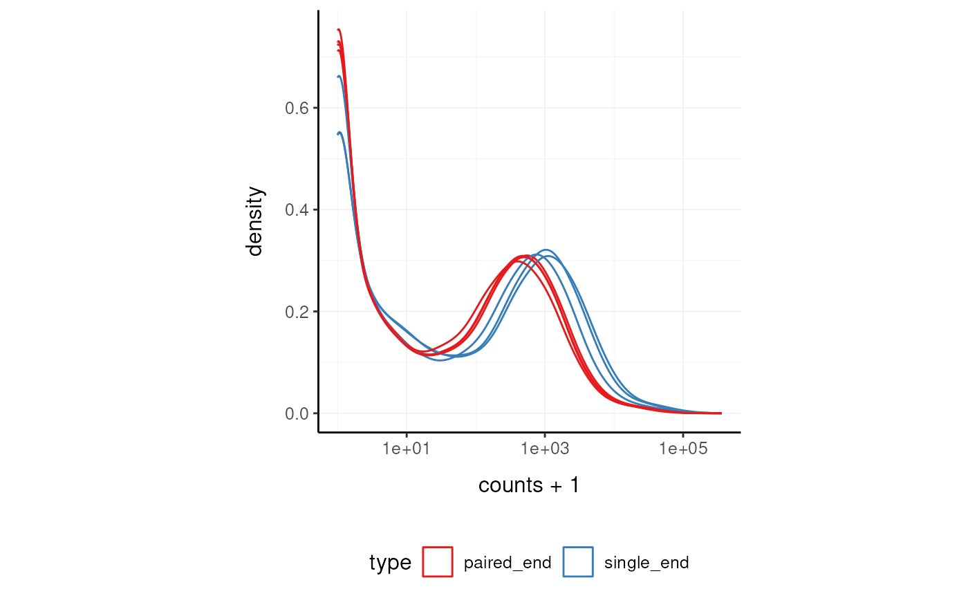
Session Info
## R Under development (unstable) (2026-03-08 r89578)
## Platform: x86_64-pc-linux-gnu
## Running under: Ubuntu 24.04.4 LTS
##
## Matrix products: default
## BLAS:   /usr/lib/x86_64-linux-gnu/openblas-pthread/libblas.so.3
## LAPACK: /usr/lib/x86_64-linux-gnu/openblas-pthread/libopenblasp-r0.3.26.so;  LAPACK version 3.12.0
##
## locale:
##  [1] LC_CTYPE=en_US.UTF-8       LC_NUMERIC=C
##  [3] LC_TIME=en_US.UTF-8        LC_COLLATE=en_US.UTF-8
##  [5] LC_MONETARY=en_US.UTF-8    LC_MESSAGES=en_US.UTF-8
##  [7] LC_PAPER=en_US.UTF-8       LC_NAME=C
##  [9] LC_ADDRESS=C               LC_TELEPHONE=C
## [11] LC_MEASUREMENT=en_US.UTF-8 LC_IDENTIFICATION=C
##
## time zone: UTC
## tzcode source: system (glibc)
##
## attached base packages:
## [1] stats4    stats     graphics  grDevices utils     datasets  methods
## [8] base
##
## other attached packages:
##  [1] tidyr_1.3.2                     tidySummarizedExperiment_1.20.3
##  [3] ttservice_0.5.3                 SummarizedExperiment_1.41.1
##  [5] Biobase_2.71.0                  GenomicRanges_1.63.1
##  [7] Seqinfo_1.1.0                   IRanges_2.45.0
##  [9] S4Vectors_0.49.0                BiocGenerics_0.57.0
## [11] generics_0.1.4                  MatrixGenerics_1.23.0
## [13] matrixStats_1.5.0               dplyr_1.2.0
## [15] ggplot2_4.0.2                   knitr_1.51
##
## loaded via a namespace (and not attached):
##  [1] gtable_0.3.6        xfun_0.56           bslib_0.10.0
##  [4] htmlwidgets_1.6.4   lattice_0.22-9      vctrs_0.7.1
##  [7] tools_4.6.0         tibble_3.3.1        pkgconfig_2.0.3
## [10] Matrix_1.7-4        data.table_1.18.2.1 RColorBrewer_1.1-3
## [13] S7_0.2.1            desc_1.4.3          lifecycle_1.0.5
## [16] compiler_4.6.0      farver_2.1.2        stringr_1.6.0
## [19] textshaping_1.0.5   prettydoc_0.4.1     htmltools_0.5.9
## [22] sass_0.4.10         yaml_2.3.12         lazyeval_0.2.2
## [25] plotly_4.12.0       pillar_1.11.1       pkgdown_2.2.0
## [28] jquerylib_0.1.4     ellipsis_0.3.2      DelayedArray_0.37.0
## [31] cachem_1.1.0        abind_1.4-8         tidyselect_1.2.1
## [34] digest_0.6.39       stringi_1.8.7       purrr_1.2.1
## [37] labeling_0.4.3      fastmap_1.2.0       grid_4.6.0
## [40] cli_3.6.5           SparseArray_1.11.11 magrittr_2.0.4
## [43] S4Arrays_1.11.1     utf8_1.2.6          withr_3.0.2
## [46] scales_1.4.0        rmarkdown_2.30      XVector_0.51.0
## [49] httr_1.4.8          otel_0.2.0          ragg_1.5.1
## [52] evaluate_1.0.5      viridisLite_0.4.3   rlang_1.1.7
## [55] glue_1.8.0          jsonlite_2.0.0      R6_2.6.1
## [58] systemfonts_1.3.2   fs_1.6.7