Tidy Transcriptomics for Single-cell RNA Sequencing Analyses with Bioconductor

Instructors

Dr. Stefano Mangiola is currently a Postdoctoral researcher in the laboratory of Prof. Tony Papenfuss at the Walter and Eliza Hall Institute in Melbourne, Australia. His background spans from biotechnology to bioinformatics and biostatistics. His research focuses on prostate and breast tumour microenvironment, the development of statistical models for the analysis of RNA sequencing data, and data analysis and visualisation interfaces.

Workshop goals and objectives

What you will learn

Basic tidy operations possible with tidyseurat and tidySingleCellExperiment
The differences between Seurat and SingleCellExperiment representation, and tidy representation
How to interface Seurat and SingleCellExperiment with tidy manipulation and visualisation
A real-world case study that will showcase the power of tidy single-cell methods compared with base/ad-hoc methods

What you will not learn

The molecular technology of single-cell sequencing
The fundamentals of single-cell data analysis
The fundamentals of tidy data analysis

Getting started

Local

We will use the Cloud during the workshop and this method is available if you want to run the material after the workshop. If you want to install on your own computer, see instructions here.

Alternatively, you can view the material at the workshop webpage here.

Introduction to tidytranscriptomics

Here

Part 1 Introduction to tidySingleCellExperiment

# Load packages
library(SingleCellExperiment)
library(ggplot2)
library(plotly)
library(dplyr)
library(colorspace)
library(dittoSeq)

SingleCellExperiment is a very popular analysis toolkit for single cell RNA sequencing data (Butler et al. 2018; Stuart et al. 2019).

Here we load single-cell data in SingleCellExperiment object format. This data is peripheral blood mononuclear cells (PBMCs) from metastatic breast cancer patients.

# load single cell RNA sequencing data
sce_obj <- tidyomicsWorkshop::sce_obj

# take a look
sce_obj

## class: SingleCellExperiment 
## dim: 482 3580 
## metadata(0):
## assays(2): counts logcounts
## rownames(482): HBB HBA2 ... TRGC2 CD8A
## rowData names(0):
## colnames(3580): 1_AAATGGACAAGTTCGT-1 1_AACAAGAGTGTTGAGG-1 ...
##   10_TTTGTTGGTACACGTT-1 10_TTTGTTGGTGATAGAT-1
## colData names(15): Barcode batch ... treatment sample
## reducedDimNames(1): UMAP
## mainExpName: SCT
## altExpNames(1): RNA

tidySingleCellExperiment provides a bridge between the SingleCellExperiment single-cell package and the tidyverse (Wickham et al. 2019). It creates an invisible layer that enables viewing the SingleCellExperiment object as a tidyverse tibble, and provides SingleCellExperiment-compatible dplyr, tidyr, ggplot and plotly functions.

If we load the tidySingleCellExperiment package and then view the single cell data, it now displays as a tibble.

library(tidySingleCellExperiment)

sce_obj

## # A SingleCellExperiment-tibble abstraction: 3,580 × 18
## # Features=482 | Cells=3580 | Assays=counts, logcounts
##    .cell       Barcode batch BCB    S.Score G2M.Score Phase cell_type nCount_RNA
##    <chr>       <fct>   <fct> <fct>    <dbl>     <dbl> <fct> <fct>          <int>
##  1 1_AAATGGAC… AAATGG… 1     BCB1… -2.07e-2   -0.0602 G1    TCR_V_De…        215
##  2 1_AACAAGAG… AACAAG… 1     BCB1…  2.09e-2   -0.0357 S     CD8+_tra…        145
##  3 1_AACGTCAG… AACGTC… 1     BCB1… -2.54e-2   -0.133  G1    CD8+_hig…        356
##  4 1_AACTTCTC… AACTTC… 1     BCB1…  2.85e-2   -0.163  S     CD8+_tra…        385
##  5 1_AAGTCGTG… AAGTCG… 1     BCB1… -2.30e-2   -0.0581 G1    MAIT             352
##  6 1_AATGAAGC… AATGAA… 1     BCB1…  1.09e-2   -0.0621 S     CD4+_rib…        335
##  7 1_ACAAAGAG… ACAAAG… 1     BCB1… -2.06e-2   -0.0409 G1    CD4+_Tcm…        242
##  8 1_ACACGCGC… ACACGC… 1     BCB1… -3.95e-4   -0.176  G1    CD8+_hig…        438
##  9 1_ACATGCAT… ACATGC… 1     BCB1… -4.09e-2   -0.0829 G1    CD4+_rib…        180
## 10 1_ACGATCAT… ACGATC… 1     BCB1…  8.82e-2   -0.0397 S     CD4+_rib…         82
## # ℹ 3,570 more rows
## # ℹ 9 more variables: nFeature_RNA <int>, nCount_SCT <int>, nFeature_SCT <int>,
## #   ident <fct>, file <chr>, treatment <chr>, sample <glue>, UMAP_1 <dbl>,
## #   UMAP_2 <dbl>

If we want to revert to the standard SingleCellExperiment view we can do that.

options("restore_SingleCellExperiment_show" = TRUE)
sce_obj

## class: SingleCellExperiment 
## dim: 482 3580 
## metadata(0):
## assays(2): counts logcounts
## rownames(482): HBB HBA2 ... TRGC2 CD8A
## rowData names(0):
## colnames(3580): 1_AAATGGACAAGTTCGT-1 1_AACAAGAGTGTTGAGG-1 ...
##   10_TTTGTTGGTACACGTT-1 10_TTTGTTGGTGATAGAT-1
## colData names(15): Barcode batch ... treatment sample

If we want to revert back to tidy SingleCellExperiment view we can.

options("restore_SingleCellExperiment_show" = FALSE)
sce_obj

## # A SingleCellExperiment-tibble abstraction: 3,580 × 18
## # Features=482 | Cells=3580 | Assays=counts, logcounts
##    .cell       Barcode batch BCB    S.Score G2M.Score Phase cell_type nCount_RNA
##    <chr>       <fct>   <fct> <fct>    <dbl>     <dbl> <fct> <fct>          <int>
##  1 1_AAATGGAC… AAATGG… 1     BCB1… -2.07e-2   -0.0602 G1    TCR_V_De…        215
##  2 1_AACAAGAG… AACAAG… 1     BCB1…  2.09e-2   -0.0357 S     CD8+_tra…        145
##  3 1_AACGTCAG… AACGTC… 1     BCB1… -2.54e-2   -0.133  G1    CD8+_hig…        356
##  4 1_AACTTCTC… AACTTC… 1     BCB1…  2.85e-2   -0.163  S     CD8+_tra…        385
##  5 1_AAGTCGTG… AAGTCG… 1     BCB1… -2.30e-2   -0.0581 G1    MAIT             352
##  6 1_AATGAAGC… AATGAA… 1     BCB1…  1.09e-2   -0.0621 S     CD4+_rib…        335
##  7 1_ACAAAGAG… ACAAAG… 1     BCB1… -2.06e-2   -0.0409 G1    CD4+_Tcm…        242
##  8 1_ACACGCGC… ACACGC… 1     BCB1… -3.95e-4   -0.176  G1    CD8+_hig…        438
##  9 1_ACATGCAT… ACATGC… 1     BCB1… -4.09e-2   -0.0829 G1    CD4+_rib…        180
## 10 1_ACGATCAT… ACGATC… 1     BCB1…  8.82e-2   -0.0397 S     CD4+_rib…         82
## # ℹ 3,570 more rows
## # ℹ 9 more variables: nFeature_RNA <int>, nCount_SCT <int>, nFeature_SCT <int>,
## #   ident <fct>, file <chr>, treatment <chr>, sample <glue>, UMAP_1 <dbl>,
## #   UMAP_2 <dbl>

It can be interacted with using SingleCellExperiment commands such as assays.

assays(sce_obj)

## List of length 2
## names(2): counts logcounts

We can also interact with our object as we do with any tidyverse tibble.

Tidyverse commands

We can use tidyverse commands, such as filter, select and mutate to explore the tidySingleCellExperiment object. Some examples are shown below and more can be seen at the tidySingleCellExperiment website here.

We can use filter to choose rows, for example, to see just the rows for the cells in G1 cell-cycle stage.

sce_obj |> filter(Phase == "G1")

## # A SingleCellExperiment-tibble abstraction: 1,859 × 18
## # Features=482 | Cells=1859 | Assays=counts, logcounts
##    .cell       Barcode batch BCB    S.Score G2M.Score Phase cell_type nCount_RNA
##    <chr>       <fct>   <fct> <fct>    <dbl>     <dbl> <fct> <fct>          <int>
##  1 1_AAATGGAC… AAATGG… 1     BCB1… -2.07e-2   -0.0602 G1    TCR_V_De…        215
##  2 1_AACGTCAG… AACGTC… 1     BCB1… -2.54e-2   -0.133  G1    CD8+_hig…        356
##  3 1_AAGTCGTG… AAGTCG… 1     BCB1… -2.30e-2   -0.0581 G1    MAIT             352
##  4 1_ACAAAGAG… ACAAAG… 1     BCB1… -2.06e-2   -0.0409 G1    CD4+_Tcm…        242
##  5 1_ACACGCGC… ACACGC… 1     BCB1… -3.95e-4   -0.176  G1    CD8+_hig…        438
##  6 1_ACATGCAT… ACATGC… 1     BCB1… -4.09e-2   -0.0829 G1    CD4+_rib…        180
##  7 1_ACGTAACG… ACGTAA… 1     BCB1… -8.69e-3   -0.140  G1    TCR_V_De…        187
##  8 1_AGAGAATT… AGAGAA… 1     BCB1… -5.14e-3   -0.102  G1    CD8+_tra…        155
##  9 1_AGATCCAT… AGATCC… 1     BCB1… -1.17e-2   -0.155  G1    CD8+_hig…        433
## 10 1_AGCCAATA… AGCCAA… 1     BCB1… -3.61e-2   -0.207  G1    CD4+_Tcm…        353
## # ℹ 1,849 more rows
## # ℹ 9 more variables: nFeature_RNA <int>, nCount_SCT <int>, nFeature_SCT <int>,
## #   ident <fct>, file <chr>, treatment <chr>, sample <glue>, UMAP_1 <dbl>,
## #   UMAP_2 <dbl>

We can use select to view columns, for example, to see the filename, total cellular RNA abundance and cell phase.

If we use select we will also get any view-only columns returned, such as the UMAP columns generated during the preprocessing.

sce_obj |> select(.cell, file, nCount_RNA, Phase)

## # A SingleCellExperiment-tibble abstraction: 3,580 × 6
## # Features=482 | Cells=3580 | Assays=counts, logcounts
##    .cell                file                      nCount_RNA Phase UMAP_1 UMAP_2
##    <chr>                <chr>                          <int> <fct>  <dbl>  <dbl>
##  1 1_AAATGGACAAGTTCGT-1 ../data/single_cell/SI-G…        215 G1    -3.73  -1.59 
##  2 1_AACAAGAGTGTTGAGG-1 ../data/single_cell/SI-G…        145 S      0.798 -0.151
##  3 1_AACGTCAGTCTATGAC-1 ../data/single_cell/SI-G…        356 G1    -0.292  0.515
##  4 1_AACTTCTCACGCTGAC-1 ../data/single_cell/SI-G…        385 S      0.372  2.34 
##  5 1_AAGTCGTGTGTTGCCG-1 ../data/single_cell/SI-G…        352 G1    -1.63  -0.236
##  6 1_AATGAAGCATCCAACA-1 ../data/single_cell/SI-G…        335 S      0.822  2.90 
##  7 1_ACAAAGAGTCGTACTA-1 ../data/single_cell/SI-G…        242 G1     3.28   3.97 
##  8 1_ACACGCGCAGGTACGA-1 ../data/single_cell/SI-G…        438 G1    -3.65  -0.192
##  9 1_ACATGCATCACTTTGT-1 ../data/single_cell/SI-G…        180 G1    -0.273  4.09 
## 10 1_ACGATCATCGACGAGA-1 ../data/single_cell/SI-G…         82 S     -0.816  2.90 
## # ℹ 3,570 more rows

We can use mutate to create a column. For example, we could create a new Phase_l column that contains a lower-case version of Phase.

sce_obj |>
  mutate(Phase_l = tolower(Phase)) |>
  select(.cell, Phase, Phase_l)

## # A SingleCellExperiment-tibble abstraction: 3,580 × 5
## # Features=482 | Cells=3580 | Assays=counts, logcounts
##    .cell                Phase Phase_l UMAP_1 UMAP_2
##    <chr>                <fct> <chr>    <dbl>  <dbl>
##  1 1_AAATGGACAAGTTCGT-1 G1    g1      -3.73  -1.59 
##  2 1_AACAAGAGTGTTGAGG-1 S     s        0.798 -0.151
##  3 1_AACGTCAGTCTATGAC-1 G1    g1      -0.292  0.515
##  4 1_AACTTCTCACGCTGAC-1 S     s        0.372  2.34 
##  5 1_AAGTCGTGTGTTGCCG-1 G1    g1      -1.63  -0.236
##  6 1_AATGAAGCATCCAACA-1 S     s        0.822  2.90 
##  7 1_ACAAAGAGTCGTACTA-1 G1    g1       3.28   3.97 
##  8 1_ACACGCGCAGGTACGA-1 G1    g1      -3.65  -0.192
##  9 1_ACATGCATCACTTTGT-1 G1    g1      -0.273  4.09 
## 10 1_ACGATCATCGACGAGA-1 S     s       -0.816  2.90 
## # ℹ 3,570 more rows

We can use tidyverse commands to polish an annotation column. We will extract the sample, and group information from the file name column into separate columns.

# First take a look at the file column
sce_obj |> select(.cell, file)

## # A SingleCellExperiment-tibble abstraction: 3,580 × 4
## # Features=482 | Cells=3580 | Assays=counts, logcounts
##    .cell                file                                       UMAP_1 UMAP_2
##    <chr>                <chr>                                       <dbl>  <dbl>
##  1 1_AAATGGACAAGTTCGT-1 ../data/single_cell/SI-GA-H1/outs/raw_fea… -3.73  -1.59 
##  2 1_AACAAGAGTGTTGAGG-1 ../data/single_cell/SI-GA-H1/outs/raw_fea…  0.798 -0.151
##  3 1_AACGTCAGTCTATGAC-1 ../data/single_cell/SI-GA-H1/outs/raw_fea… -0.292  0.515
##  4 1_AACTTCTCACGCTGAC-1 ../data/single_cell/SI-GA-H1/outs/raw_fea…  0.372  2.34 
##  5 1_AAGTCGTGTGTTGCCG-1 ../data/single_cell/SI-GA-H1/outs/raw_fea… -1.63  -0.236
##  6 1_AATGAAGCATCCAACA-1 ../data/single_cell/SI-GA-H1/outs/raw_fea…  0.822  2.90 
##  7 1_ACAAAGAGTCGTACTA-1 ../data/single_cell/SI-GA-H1/outs/raw_fea…  3.28   3.97 
##  8 1_ACACGCGCAGGTACGA-1 ../data/single_cell/SI-GA-H1/outs/raw_fea… -3.65  -0.192
##  9 1_ACATGCATCACTTTGT-1 ../data/single_cell/SI-GA-H1/outs/raw_fea… -0.273  4.09 
## 10 1_ACGATCATCGACGAGA-1 ../data/single_cell/SI-GA-H1/outs/raw_fea… -0.816  2.90 
## # ℹ 3,570 more rows

# Create column for sample
sce_obj <- sce_obj |>
  # Extract sample
  extract(file, "sample", "../data/.*/([a-zA-Z0-9_-]+)/outs.+", remove = FALSE)

# Take a look
sce_obj |> select(.cell, sample, everything())

## # A SingleCellExperiment-tibble abstraction: 3,580 × 18
## # Features=482 | Cells=3580 | Assays=counts, logcounts
##    .cell           sample Barcode batch BCB    S.Score G2M.Score Phase cell_type
##    <chr>           <chr>  <fct>   <fct> <fct>    <dbl>     <dbl> <fct> <fct>    
##  1 1_AAATGGACAAGT… SI-GA… AAATGG… 1     BCB1… -2.07e-2   -0.0602 G1    TCR_V_De…
##  2 1_AACAAGAGTGTT… SI-GA… AACAAG… 1     BCB1…  2.09e-2   -0.0357 S     CD8+_tra…
##  3 1_AACGTCAGTCTA… SI-GA… AACGTC… 1     BCB1… -2.54e-2   -0.133  G1    CD8+_hig…
##  4 1_AACTTCTCACGC… SI-GA… AACTTC… 1     BCB1…  2.85e-2   -0.163  S     CD8+_tra…
##  5 1_AAGTCGTGTGTT… SI-GA… AAGTCG… 1     BCB1… -2.30e-2   -0.0581 G1    MAIT     
##  6 1_AATGAAGCATCC… SI-GA… AATGAA… 1     BCB1…  1.09e-2   -0.0621 S     CD4+_rib…
##  7 1_ACAAAGAGTCGT… SI-GA… ACAAAG… 1     BCB1… -2.06e-2   -0.0409 G1    CD4+_Tcm…
##  8 1_ACACGCGCAGGT… SI-GA… ACACGC… 1     BCB1… -3.95e-4   -0.176  G1    CD8+_hig…
##  9 1_ACATGCATCACT… SI-GA… ACATGC… 1     BCB1… -4.09e-2   -0.0829 G1    CD4+_rib…
## 10 1_ACGATCATCGAC… SI-GA… ACGATC… 1     BCB1…  8.82e-2   -0.0397 S     CD4+_rib…
## # ℹ 3,570 more rows
## # ℹ 9 more variables: nCount_RNA <int>, nFeature_RNA <int>, nCount_SCT <int>,
## #   nFeature_SCT <int>, ident <fct>, file <chr>, treatment <chr>, UMAP_1 <dbl>,
## #   UMAP_2 <dbl>

We could use tidyverse unite to combine columns, for example to create a new column for sample id combining the sample and patient id (BCB) columns.

sce_obj <- sce_obj |> unite("sample_id", sample, BCB, remove = FALSE)

# Take a look
sce_obj |> select(.cell, sample_id, sample, BCB)

## # A SingleCellExperiment-tibble abstraction: 3,580 × 6
## # Features=482 | Cells=3580 | Assays=counts, logcounts
##    .cell                sample_id       sample   BCB    UMAP_1 UMAP_2
##    <chr>                <chr>           <chr>    <fct>   <dbl>  <dbl>
##  1 1_AAATGGACAAGTTCGT-1 SI-GA-H1_BCB102 SI-GA-H1 BCB102 -3.73  -1.59 
##  2 1_AACAAGAGTGTTGAGG-1 SI-GA-H1_BCB102 SI-GA-H1 BCB102  0.798 -0.151
##  3 1_AACGTCAGTCTATGAC-1 SI-GA-H1_BCB102 SI-GA-H1 BCB102 -0.292  0.515
##  4 1_AACTTCTCACGCTGAC-1 SI-GA-H1_BCB102 SI-GA-H1 BCB102  0.372  2.34 
##  5 1_AAGTCGTGTGTTGCCG-1 SI-GA-H1_BCB102 SI-GA-H1 BCB102 -1.63  -0.236
##  6 1_AATGAAGCATCCAACA-1 SI-GA-H1_BCB102 SI-GA-H1 BCB102  0.822  2.90 
##  7 1_ACAAAGAGTCGTACTA-1 SI-GA-H1_BCB102 SI-GA-H1 BCB102  3.28   3.97 
##  8 1_ACACGCGCAGGTACGA-1 SI-GA-H1_BCB102 SI-GA-H1 BCB102 -3.65  -0.192
##  9 1_ACATGCATCACTTTGT-1 SI-GA-H1_BCB102 SI-GA-H1 BCB102 -0.273  4.09 
## 10 1_ACGATCATCGACGAGA-1 SI-GA-H1_BCB102 SI-GA-H1 BCB102 -0.816  2.90 
## # ℹ 3,570 more rows

Part 2 Signature visualisation

Data pre-processing

The object sce_obj we’ve been using was created as part of a study on breast cancer systemic immune response. Peripheral blood mononuclear cells have been sequenced for RNA at the single-cell level. The steps used to generate the object are summarised below.

scran, scater, and DropletsUtils packages have been used to eliminate empty droplets and dead cells. Samples were individually quality checked and cells were filtered for good gene coverage.
Variable features were identified using modelGeneVar.
Read counts were scaled and normalised using logNormCounts from scuttle.
Data integration was performed using fastMNN with default parameters.
PCA performed to reduce feature dimensionality.
Nearest-neighbor cell networks were calculated using 30 principal components.
2 UMAP dimensions were calculated using 30 principal components.
Cells with similar transcriptome profiles were grouped into clusters using Louvain clustering from scran.

Analyse custom signature

The researcher analysing this dataset wanted to identify gamma delta T cells using a gene signature from a published paper (Pizzolato et al. 2019). We’ll show how that can be done here.

With tidySingleCellExperiment’s join_features we can view the counts for genes in the signature as columns joined to our single cell tibble.

sce_obj |>
  join_features(c("CD3D", "TRDC", "TRGC1", "TRGC2", "CD8A", "CD8B"), shape = "wide")

## # A SingleCellExperiment-tibble abstraction: 3,580 × 25
## # Features=482 | Cells=3580 | Assays=counts, logcounts
##    .cell        Barcode batch sample_id BCB    S.Score G2M.Score Phase cell_type
##    <chr>        <fct>   <fct> <chr>     <fct>    <dbl>     <dbl> <fct> <fct>    
##  1 1_AAATGGACA… AAATGG… 1     SI-GA-H1… BCB1… -2.07e-2   -0.0602 G1    TCR_V_De…
##  2 1_AACAAGAGT… AACAAG… 1     SI-GA-H1… BCB1…  2.09e-2   -0.0357 S     CD8+_tra…
##  3 1_AACGTCAGT… AACGTC… 1     SI-GA-H1… BCB1… -2.54e-2   -0.133  G1    CD8+_hig…
##  4 1_AACTTCTCA… AACTTC… 1     SI-GA-H1… BCB1…  2.85e-2   -0.163  S     CD8+_tra…
##  5 1_AAGTCGTGT… AAGTCG… 1     SI-GA-H1… BCB1… -2.30e-2   -0.0581 G1    MAIT     
##  6 1_AATGAAGCA… AATGAA… 1     SI-GA-H1… BCB1…  1.09e-2   -0.0621 S     CD4+_rib…
##  7 1_ACAAAGAGT… ACAAAG… 1     SI-GA-H1… BCB1… -2.06e-2   -0.0409 G1    CD4+_Tcm…
##  8 1_ACACGCGCA… ACACGC… 1     SI-GA-H1… BCB1… -3.95e-4   -0.176  G1    CD8+_hig…
##  9 1_ACATGCATC… ACATGC… 1     SI-GA-H1… BCB1… -4.09e-2   -0.0829 G1    CD4+_rib…
## 10 1_ACGATCATC… ACGATC… 1     SI-GA-H1… BCB1…  8.82e-2   -0.0397 S     CD4+_rib…
## # ℹ 3,570 more rows
## # ℹ 16 more variables: nCount_RNA <int>, nFeature_RNA <int>, nCount_SCT <int>,
## #   nFeature_SCT <int>, ident <fct>, file <chr>, sample <chr>, treatment <chr>,
## #   CD3D <dbl>, TRDC <dbl>, TRGC1 <dbl>, TRGC2 <dbl>, CD8A <dbl>, CD8B <dbl>,
## #   UMAP_1 <dbl>, UMAP_2 <dbl>

We can use tidyverse mutate to create a column containing the signature score. To generate the score, we scale the sum of the 4 genes, CD3D, TRDC, TRGC1, TRGC2, and subtract the scaled sum of the 2 genes, CD8A and CD8B. mutate is powerful in enabling us to perform complex arithmetic operations easily.

sce_obj |>
    
  join_features(c("CD3D", "TRDC", "TRGC1", "TRGC2", "CD8A", "CD8B"), shape = "wide") |>
    
  mutate(
    signature_score =
      scales::rescale(CD3D + TRDC + TRGC1 + TRGC2, to = c(0, 1)) -
        scales::rescale(CD8A + CD8B, to = c(0, 1))
  ) |>
    
  select(.cell, signature_score, everything())

## # A SingleCellExperiment-tibble abstraction: 3,580 × 26
## # Features=482 | Cells=3580 | Assays=counts, logcounts
##    .cell  signature_score Barcode batch sample_id BCB    S.Score G2M.Score Phase
##    <chr>            <dbl> <fct>   <fct> <chr>     <fct>    <dbl>     <dbl> <fct>
##  1 1_AAA…          0.386  AAATGG… 1     SI-GA-H1… BCB1… -2.07e-2   -0.0602 G1   
##  2 1_AAC…          0.108  AACAAG… 1     SI-GA-H1… BCB1…  2.09e-2   -0.0357 S    
##  3 1_AAC…         -0.789  AACGTC… 1     SI-GA-H1… BCB1… -2.54e-2   -0.133  G1   
##  4 1_AAC…         -0.0694 AACTTC… 1     SI-GA-H1… BCB1…  2.85e-2   -0.163  S    
##  5 1_AAG…          0      AAGTCG… 1     SI-GA-H1… BCB1… -2.30e-2   -0.0581 G1   
##  6 1_AAT…          0      AATGAA… 1     SI-GA-H1… BCB1…  1.09e-2   -0.0621 S    
##  7 1_ACA…          0.108  ACAAAG… 1     SI-GA-H1… BCB1… -2.06e-2   -0.0409 G1   
##  8 1_ACA…          0.170  ACACGC… 1     SI-GA-H1… BCB1… -3.95e-4   -0.176  G1   
##  9 1_ACA…          0      ACATGC… 1     SI-GA-H1… BCB1… -4.09e-2   -0.0829 G1   
## 10 1_ACG…          0.278  ACGATC… 1     SI-GA-H1… BCB1…  8.82e-2   -0.0397 S    
## # ℹ 3,570 more rows
## # ℹ 17 more variables: cell_type <fct>, nCount_RNA <int>, nFeature_RNA <int>,
## #   nCount_SCT <int>, nFeature_SCT <int>, ident <fct>, file <chr>,
## #   sample <chr>, treatment <chr>, CD3D <dbl>, TRDC <dbl>, TRGC1 <dbl>,
## #   TRGC2 <dbl>, CD8A <dbl>, CD8B <dbl>, UMAP_1 <dbl>, UMAP_2 <dbl>

The gamma delta T cells could then be visualised by the signature score using Bioconductor’s visualisation functions.

sce_obj |>
    
  join_features(
    features = c("CD3D", "TRDC", "TRGC1", "TRGC2", "CD8A", "CD8B"), shape = "wide"
  ) |>
    
  mutate(
    signature_score =
      scales::rescale(CD3D + TRDC + TRGC1 + TRGC2, to = c(0, 1)) -
        scales::rescale(CD8A + CD8B, to = c(0, 1))
  ) |>
    
  scater::plotUMAP(colour_by = "signature_score")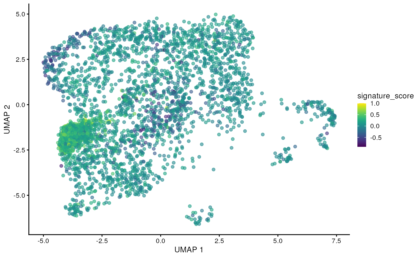

The cells could also be visualised using the popular and powerful ggplot2 package, enabling the researcher to use ggplot functions they were familiar with, and to customise the plot with great flexibility.

sce_obj |>
    
  join_features(
    features = c("CD3D", "TRDC", "TRGC1", "TRGC2", "CD8A", "CD8B"), shape = "wide"
  ) |>
    
  mutate(
    signature_score =
      scales::rescale(CD3D + TRDC + TRGC1 + TRGC2, to = c(0, 1)) -
        scales::rescale(CD8A + CD8B, to = c(0, 1))
  ) |>
    
  # plot cells with high score last so they're not obscured by other cells
  arrange(signature_score) |>
    
  ggplot(aes(UMAP_1, UMAP_2, color = signature_score)) +
  geom_point() +
  scale_color_distiller(palette = "Spectral") +
  tidyomicsWorkshop::theme_multipanel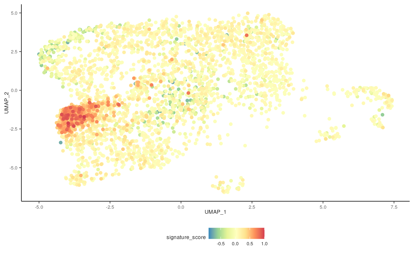

For exploratory analyses, we can select the gamma delta T cells, the red cluster on the left with high signature score. We’ll filter for cells with a signature score > 0.7.

sce_obj_gamma_delta <-
    
  sce_obj |>
    
  join_features(
    features = c("CD3D", "TRDC", "TRGC1", "TRGC2", "CD8A", "CD8B"), shape = "wide"
  ) |>
    
  mutate(
    signature_score =
      scales::rescale(CD3D + TRDC + TRGC1 + TRGC2, to = c(0, 1)) -
        scales::rescale(CD8A + CD8B, to = c(0, 1))
  ) |>
    
    # Proper cluster selection should be used instead (see supplementary material)
  filter(signature_score > 0.7)

For comparison, we show the alternative using base R and SingleCellExperiment. Note that the code contains more redundancy and intermediate objects.

counts_positive <-
  assay(sce_obj, "logcounts")[c("CD3D", "TRDC", "TRGC1", "TRGC2"), ] |>
  colSums() |>
  scales::rescale(to = c(0, 1))

counts_negative <-
  assay(sce_obj, "logcounts")[c("CD8A", "CD8B"), ] |>
  colSums() |>
  scales::rescale(to = c(0, 1))

sce_obj$signature_score <- counts_positive - counts_negative

sce_obj_gamma_delta <- sce_obj[, sce_obj$signature_score > 0.7]

We can then focus on just these gamma delta T cells and chain Bioconductor and tidyverse commands together to analyse.

library(batchelor)
library(scater)

sce_obj_gamma_delta <-
    
  sce_obj_gamma_delta |>
    
  # Integrate - using batchelor.
  multiBatchNorm(batch = colData(sce_obj_gamma_delta)$sample) |>
  fastMNN(batch = colData(sce_obj_gamma_delta)$sample) |>
    
  # Join metadata removed by fastMNN - using tidyverse
  left_join(as_tibble(sce_obj_gamma_delta)) |>
    
  # Dimension reduction - using scater
  runUMAP(ncomponents = 2, dimred = "corrected")

Visualise gamma delta T cells. As we have used rough threshold we are left with only few cells. Proper cluster selection should be used instead (see supplementary material).

sce_obj_gamma_delta |> plotUMAP()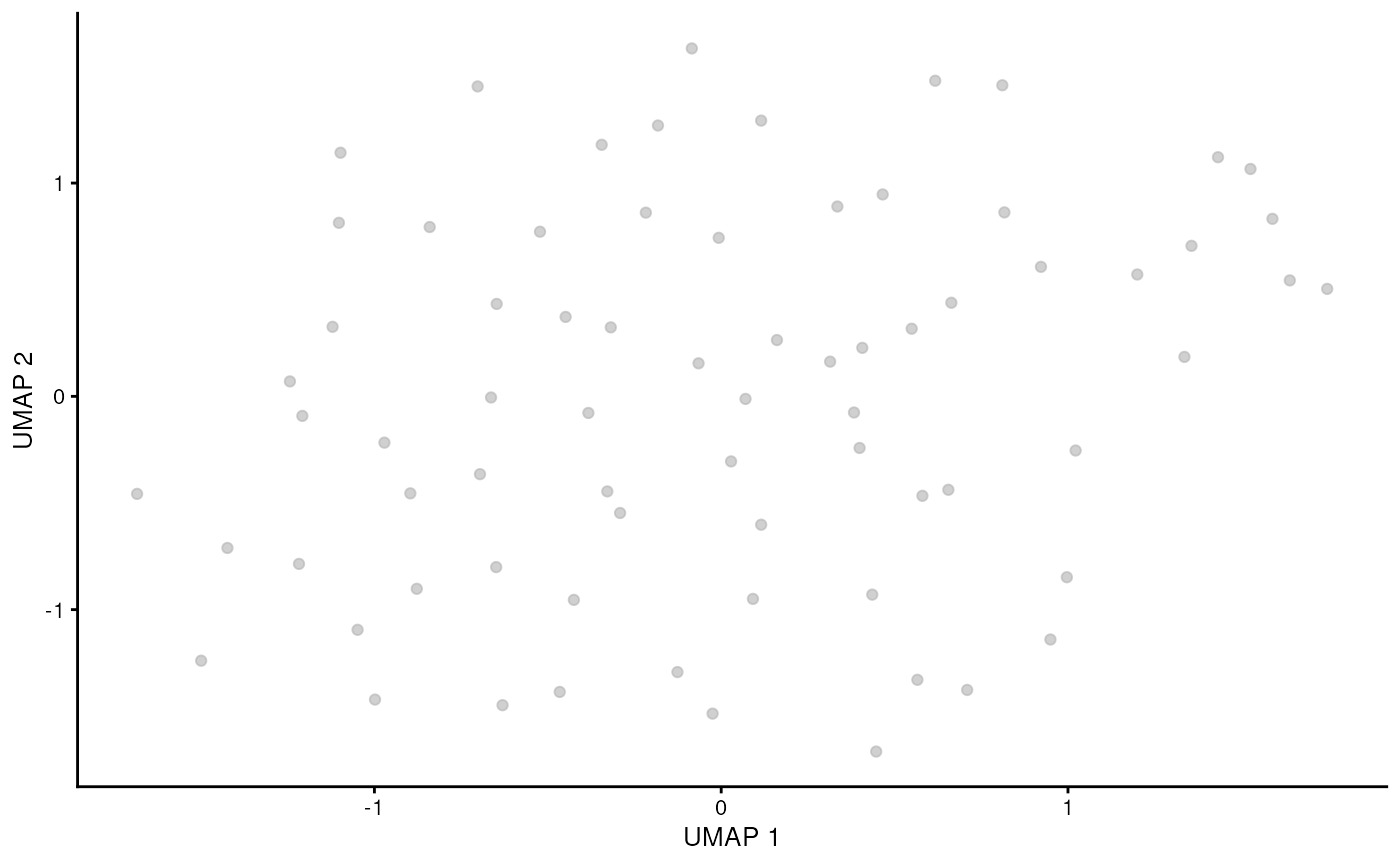

It is also possible to visualise the cells as a 3D plot using plotly. The example data used here only contains a few genes, for the sake of time and size in this demonstration, but below is how you could generate the 3 dimensions needed for 3D plot with a full dataset.

single_cell_object |>
  RunUMAP(dims = 1:30, n.components = 3L, spread = 0.5, min.dist = 0.01, n.neighbors = 10L)

We’ll demonstrate creating a 3D plot using some data that has 3 UMAP dimensions. This is a fantastic way to visualise both reduced dimensions and metadata in the same representation.

pbmc <- tidyomicsWorkshop::sce_obj_UMAP3

pbmc |>
  plot_ly(
    x = ~`UMAP_1`,
    y = ~`UMAP_2`,
    z = ~`UMAP_3`,
    color = ~cell_type,
    colors = dittoSeq::dittoColors()
  ) %>%
  add_markers(size = I(1))

Exercises

Using the sce_obj:

What proportion of all cells are gamma-delta T cells? Use signature_score > 0.7 to identify gamma-delta T cells.
There is a cluster of cells characterised by a low RNA output (nCount_RNA < 100). Identify the cell composition (cell_type) of that cluster.

Part 3 Nested analyses

When analysing single cell data is sometimes necessary to perform calculations on data subsets. For example, we might want to estimate difference in mRNA abundance between two condition for each cell type.

tidyr and purrr offer a great tool to perform iterativre analyses in a functional way.

We use tidyverse nest to group the data. The command below will create a tibble containing a column with a SummarizedExperiment object for each cell type. nest is similar to tidyverse group_by, except with nest each group is stored in a single row, and can be a complex object such as SingleCellExperiment.

Let’s import some libraries

library(purrr)

## 
## Attaching package: 'purrr'

## The following object is masked from 'package:GenomicRanges':
## 
##     reduce

## The following object is masked from 'package:IRanges':
## 
##     reduce

First let’s have a look to the cell types that constitute this dataset

sce_obj |> 
  count(cell_type)

## tidySingleCellExperiment says: A data frame is returned for independent data analysis.

## # A tibble: 13 × 2
##    cell_type                                       n
##    <fct>                                       <int>
##  1 CD4+_ribosome_rich                            299
##  2 CD4+_Tcm_S100A4_IL32_IL7R_VIM                 407
##  3 CD8+_high_ribonucleosome                      404
##  4 CD8+_Tcm                                      277
##  5 CD8+_transitional_effector_GZMK_KLRB1_LYAR4   343
##  6 HSC_lymphoid_myeloid_like                     116
##  7 limphoid_myeloid_like_HLA_CD74                 26
##  8 MAIT                                          164
##  9 NK_cells                                      337
## 10 NK_cycling                                     28
## 11 T_cell:CD8+_other                             173
## 12 TCR_V_Delta_1                                 651
## 13 TCR_V_Delta_2                                 355

Let’s group the cells based on cell identity using nest

sce_obj_nested = 
  sce_obj |> 
  nest(sce = -cell_type) 

sce_obj_nested

## # A tibble: 13 × 2
##    cell_type                                   sce             
##    <fct>                                       <list>          
##  1 TCR_V_Delta_2                               <SnglCllE[,355]>
##  2 CD8+_transitional_effector_GZMK_KLRB1_LYAR4 <SnglCllE[,343]>
##  3 CD8+_high_ribonucleosome                    <SnglCllE[,404]>
##  4 MAIT                                        <SnglCllE[,164]>
##  5 CD4+_ribosome_rich                          <SnglCllE[,299]>
##  6 CD4+_Tcm_S100A4_IL32_IL7R_VIM               <SnglCllE[,407]>
##  7 NK_cells                                    <SnglCllE[,337]>
##  8 TCR_V_Delta_1                               <SnglCllE[,651]>
##  9 HSC_lymphoid_myeloid_like                   <SnglCllE[,116]>
## 10 T_cell:CD8+_other                           <SnglCllE[,173]>
## 11 NK_cycling                                  <SnglCllE[,28]> 
## 12 CD8+_Tcm                                    <SnglCllE[,277]>
## 13 limphoid_myeloid_like_HLA_CD74              <SnglCllE[,26]>

Let’s see what the first element of the Surat column looks like

sce_obj_nested |> 
  slice(1) |> 
  pull(sce)

## [[1]]
## # A SingleCellExperiment-tibble abstraction: 355 × 18
## # Features=482 | Cells=355 | Assays=counts, logcounts
##    .cell       Barcode batch sample_id BCB    S.Score G2M.Score Phase nCount_RNA
##    <chr>       <fct>   <fct> <chr>     <fct>    <dbl>     <dbl> <fct>      <int>
##  1 1_AAATGGAC… AAATGG… 1     SI-GA-H1… BCB1… -0.0207    -0.0602 G1           215
##  2 1_ATCACGAG… ATCACG… 1     SI-GA-H1… BCB1…  0.0103    -0.109  S            271
##  3 1_ATCGCCTC… ATCGCC… 1     SI-GA-H1… BCB1… -0.0241    -0.196  G1           640
##  4 1_CGATGGCT… CGATGG… 1     SI-GA-H1… BCB1… -0.0628    -0.213  G1           495
##  5 1_CGTGCTTG… CGTGCT… 1     SI-GA-H1… BCB1… -0.0403    -0.0371 G1           158
##  6 1_CTTGAGAA… CTTGAG… 1     SI-GA-H1… BCB1…  0.00494   -0.0548 S            173
##  7 1_GAGTGTTA… GAGTGT… 1     SI-GA-H1… BCB1…  0.0109    -0.0760 S            187
##  8 1_GTACAGTG… GTACAG… 1     SI-GA-H1… BCB1…  0.0265    -0.0922 S            186
##  9 1_TTCCTTCT… TTCCTT… 1     SI-GA-H1… BCB1… -0.00800   -0.0796 G1          1881
## 10 2_AAGACTCA… AAGACT… 1     SI-GA-H3… BCB1… -0.0350    -0.0878 G1           241
## # ℹ 345 more rows
## # ℹ 9 more variables: nFeature_RNA <int>, nCount_SCT <int>, nFeature_SCT <int>,
## #   ident <fct>, file <chr>, sample <chr>, treatment <chr>, UMAP_1 <dbl>,
## #   UMAP_2 <dbl>

Now, let’s perform a differential gene-transcript abundance analysis between the two conditions for each cell type.

sce_obj_nested = 
  sce_obj_nested |> 
  
  # Filter for sample with more than 30 cells
  mutate(sce = map(sce, ~ .x |> add_count(sample) |> filter(n > 50))) |>
  filter(map_int(sce, ncol) > 0) |>

  # Select significant genes
  mutate(sce = imap(
    sce,
    ~ .x %>% {print(.y); (.)} |> 
    
    # Integrate - using batchelor.
    multiBatchNorm(batch = colData(.x)$sample) |>
    fastMNN(batch = colData(.x)$sample) |>
      
    # Join metadata removed by fastMNN - using tidyverse
    left_join(as_tibble(.x)) |>
      
    # Dimension reduction - using scater
    runUMAP(ncomponents = 2, dimred = "corrected")
  
  ))

## [1] 1
## [1] 2
## [1] 3
## [1] 4
## [1] 5
## [1] 6
## [1] 7
## [1] 8
## [1] 9

## Warning: There were 2 warnings in `mutate()`.
## The first warning was:
## ℹ In argument: `sce = imap(...)`.
## Caused by warning:
## ! You're computing too large a percentage of total singular values, use a standard svd instead.
## ℹ Run `dplyr::last_dplyr_warnings()` to see the 1 remaining warning.

sce_obj_nested

## # A tibble: 9 × 2
##   cell_type                                   sce             
##   <fct>                                       <list>          
## 1 TCR_V_Delta_2                               <SnglCllE[,234]>
## 2 CD8+_transitional_effector_GZMK_KLRB1_LYAR4 <SnglCllE[,177]>
## 3 CD8+_high_ribonucleosome                    <SnglCllE[,218]>
## 4 CD4+_ribosome_rich                          <SnglCllE[,57]> 
## 5 CD4+_Tcm_S100A4_IL32_IL7R_VIM               <SnglCllE[,211]>
## 6 NK_cells                                    <SnglCllE[,170]>
## 7 TCR_V_Delta_1                               <SnglCllE[,478]>
## 8 HSC_lymphoid_myeloid_like                   <SnglCllE[,89]> 
## 9 CD8+_Tcm                                    <SnglCllE[,269]>

We can the lies the top genes with the heat map iteratively across the cell types

sce_obj_nested = 
  sce_obj_nested |> 
  
  # Build heatmaps
  mutate(umap = map(sce,plotUMAP)) 

sce_obj_nested

## # A tibble: 9 × 3
##   cell_type                                   sce              umap  
##   <fct>                                       <list>           <list>
## 1 TCR_V_Delta_2                               <SnglCllE[,234]> <gg>  
## 2 CD8+_transitional_effector_GZMK_KLRB1_LYAR4 <SnglCllE[,177]> <gg>  
## 3 CD8+_high_ribonucleosome                    <SnglCllE[,218]> <gg>  
## 4 CD4+_ribosome_rich                          <SnglCllE[,57]>  <gg>  
## 5 CD4+_Tcm_S100A4_IL32_IL7R_VIM               <SnglCllE[,211]> <gg>  
## 6 NK_cells                                    <SnglCllE[,170]> <gg>  
## 7 TCR_V_Delta_1                               <SnglCllE[,478]> <gg>  
## 8 HSC_lymphoid_myeloid_like                   <SnglCllE[,89]>  <gg>  
## 9 CD8+_Tcm                                    <SnglCllE[,269]> <gg>

Let’s have a look to the first heatmap

sce_obj_nested |> 
  slice(1) |> 
  pull(umap)

## [[1]]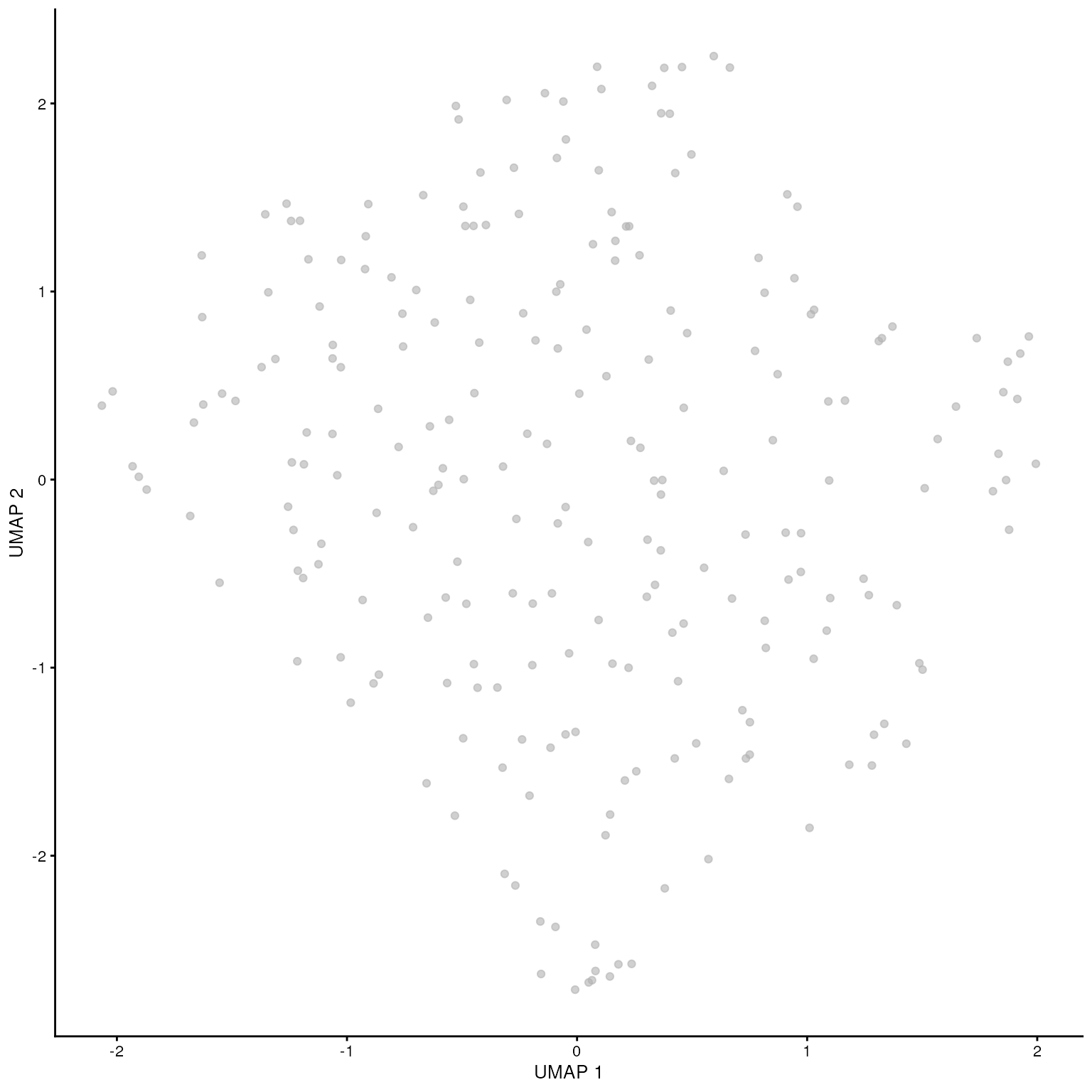

You can do this whole analysis without saving any temporary variable using the piping functionality of tidy R programming

sce_obj |> 
  
  # Nest
  nest(sce = -cell_type) |> 
  
  # Filter for sample with more than 30 cells
  mutate(sce = map(sce, ~ .x |> add_count(sample) |> filter(n > 50))) |>
  filter(map_int(sce, ncol) > 0) |>

  # Select significant genes
  mutate(sce = imap(
    sce,
    ~ .x %>% {print(.y); (.)} |> 
    
    # Integrate - using batchelor.
    multiBatchNorm(batch = colData(.x)$sample) |>
    fastMNN(batch = colData(.x)$sample) |>
      
    # Join metadata removed by fastMNN - using tidyverse
    left_join(as_tibble(.x)) |>
      
    # Dimension reduction - using scater
    runUMAP(ncomponents = 2, dimred = "corrected")
  
  )) |>
  
   # Build heatmaps
  mutate(umap = map(sce,plotUMAP))  |> 
  
  # Extract heatmaps
  pull(umap)

Exercises

Let’s suppose that you want to perform the analyses only for cell types that have a total number of cells bigger than 1000. For example, if a cell type has less than a sum of 1000 cells across all samples, that cell type will be dropped from the dataset.

Answer this question avoiding to save temporary variables, and using the function add_count to count the cells (before nesting), and then filter
Answer this question avoiding to save temporary variables, and using the function map_int to count the cells (after nesting), and the filter

Session Information

sessionInfo()

## R version 4.3.1 (2023-06-16)
## Platform: x86_64-pc-linux-gnu (64-bit)
## Running under: Ubuntu 22.04.2 LTS
## 
## Matrix products: default
## BLAS:   /usr/lib/x86_64-linux-gnu/openblas-pthread/libblas.so.3 
## LAPACK: /usr/lib/x86_64-linux-gnu/openblas-pthread/libopenblasp-r0.3.20.so;  LAPACK version 3.10.0
## 
## locale:
##  [1] LC_CTYPE=en_US.UTF-8       LC_NUMERIC=C              
##  [3] LC_TIME=en_US.UTF-8        LC_COLLATE=en_US.UTF-8    
##  [5] LC_MONETARY=en_US.UTF-8    LC_MESSAGES=en_US.UTF-8   
##  [7] LC_PAPER=en_US.UTF-8       LC_NAME=C                 
##  [9] LC_ADDRESS=C               LC_TELEPHONE=C            
## [11] LC_MEASUREMENT=en_US.UTF-8 LC_IDENTIFICATION=C       
## 
## time zone: UTC
## tzcode source: system (glibc)
## 
## attached base packages:
## [1] stats4    stats     graphics  grDevices utils     datasets  methods  
## [8] base     
## 
## other attached packages:
##  [1] purrr_1.0.1                     scater_1.28.0                  
##  [3] scuttle_1.10.1                  batchelor_1.16.0               
##  [5] tidySingleCellExperiment_1.10.0 ttservice_0.3.6                
##  [7] dittoSeq_1.12.0                 colorspace_2.1-0               
##  [9] dplyr_1.1.2                     plotly_4.10.2                  
## [11] ggplot2_3.4.2                   SingleCellExperiment_1.22.0    
## [13] SummarizedExperiment_1.30.2     Biobase_2.60.0                 
## [15] GenomicRanges_1.52.0            GenomeInfoDb_1.36.1            
## [17] IRanges_2.34.1                  S4Vectors_0.38.1               
## [19] BiocGenerics_0.46.0             MatrixGenerics_1.12.2          
## [21] matrixStats_1.0.0              
## 
## loaded via a namespace (and not attached):
##  [1] bitops_1.0-7              gridExtra_2.3            
##  [3] rlang_1.1.1               magrittr_2.0.3           
##  [5] ggridges_0.5.4            compiler_4.3.1           
##  [7] DelayedMatrixStats_1.22.1 systemfonts_1.0.4        
##  [9] vctrs_0.6.3               stringr_1.5.0            
## [11] pkgconfig_2.0.3           crayon_1.5.2             
## [13] fastmap_1.1.1             XVector_0.40.0           
## [15] ellipsis_0.3.2            labeling_0.4.2           
## [17] utf8_1.2.3                rmarkdown_2.23           
## [19] ggbeeswarm_0.7.2          ragg_1.2.5               
## [21] xfun_0.39                 zlibbioc_1.46.0          
## [23] cachem_1.0.8              beachmat_2.16.0          
## [25] jsonlite_1.8.7            highr_0.10               
## [27] DelayedArray_0.26.6       BiocParallel_1.34.2      
## [29] irlba_2.3.5.1             parallel_4.3.1           
## [31] R6_2.5.1                  bslib_0.5.0              
## [33] stringi_1.7.12            RColorBrewer_1.1-3       
## [35] jquerylib_0.1.4           Rcpp_1.0.10              
## [37] knitr_1.43                FNN_1.1.3.2              
## [39] igraph_1.5.0              Matrix_1.5-4.1           
## [41] tidyselect_1.2.0          viridis_0.6.3            
## [43] yaml_2.3.7                codetools_0.2-19         
## [45] tidyomicsWorkshop_0.16.2  lattice_0.21-8           
## [47] tibble_3.2.1              withr_2.5.0              
## [49] evaluate_0.21             desc_1.4.2               
## [51] pillar_1.9.0              generics_0.1.3           
## [53] rprojroot_2.0.3           RCurl_1.98-1.12          
## [55] sparseMatrixStats_1.12.2  munsell_0.5.0            
## [57] scales_1.2.1              glue_1.6.2               
## [59] pheatmap_1.0.12           lazyeval_0.2.2           
## [61] tools_4.3.1               BiocNeighbors_1.18.0     
## [63] data.table_1.14.8         ScaledMatrix_1.8.1       
## [65] fs_1.6.2                  cowplot_1.1.1            
## [67] grid_4.3.1                tidyr_1.3.0              
## [69] crosstalk_1.2.0           GenomeInfoDbData_1.2.10  
## [71] beeswarm_0.4.0            BiocSingular_1.16.0      
## [73] vipor_0.4.5               cli_3.6.1                
## [75] rsvd_1.0.5                textshaping_0.3.6        
## [77] fansi_1.0.4               S4Arrays_1.0.4           
## [79] viridisLite_0.4.2         uwot_0.1.16              
## [81] ResidualMatrix_1.10.0     gtable_0.3.3             
## [83] sass_0.4.6                digest_0.6.32            
## [85] ggrepel_0.9.3             farver_2.1.1             
## [87] htmlwidgets_1.6.2         memoise_2.0.1            
## [89] htmltools_0.5.5           pkgdown_2.0.7            
## [91] lifecycle_1.0.3           httr_1.4.6

References

Butler, Andrew, Paul Hoffman, Peter Smibert, Efthymia Papalexi, and Rahul Satija. 2018. “Integrating Single-Cell Transcriptomic Data Across Different Conditions, Technologies, and Species.” Nature Biotechnology 36 (5): 411–20.

Pizzolato, Gabriele, Hannah Kaminski, Marie Tosolini, Don-Marc Franchini, Fréderic Pont, Fréderic Martins, Carine Valle, et al. 2019. “Single-Cell RNA Sequencing Unveils the Shared and the Distinct Cytotoxic Hallmarks of Human TCRV\(\updelta\)1 and TCRV\(\updelta\)2 \(\upgamma\)\(\updelta\) t Lymphocytes.” Proceedings of the National Academy of Sciences, May, 201818488. https://doi.org/10.1073/pnas.1818488116.

Stuart, Tim, Andrew Butler, Paul Hoffman, Christoph Hafemeister, Efthymia Papalexi, William M Mauck III, Yuhan Hao, Marlon Stoeckius, Peter Smibert, and Rahul Satija. 2019. “Comprehensive Integration of Single-Cell Data.” Cell 177 (7): 1888–1902.

Wickham, Hadley, Mara Averick, Jennifer Bryan, Winston Chang, Lucy D’Agostino McGowan, Romain François, Garrett Grolemund, et al. 2019. “Welcome to the Tidyverse.” Journal of Open Source Software 4 (43): 1686.

<maria.doyle at petermac.org>↩︎
<mangiola.s at wehi.edu.au>↩︎

Maria Doyle, Peter MacCallum Cancer Centre¹

Stefano Mangiola, Walter and Eliza Hall Institute²

Instructors

Workshop goals and objectives

What you will learn

What you will not learn

Getting started

Local

Introduction to tidytranscriptomics

Part 1 Introduction to tidySingleCellExperiment

Tidyverse commands

Part 2 Signature visualisation

Data pre-processing

Analyse custom signature

Exercises

Part 3 Nested analyses

Exercises

Tidy Transcriptomics for Single-cell RNA Sequencing Analyses with Bioconductor

Maria Doyle, Peter MacCallum Cancer Centre1

Stefano Mangiola, Walter and Eliza Hall Institute2

Instructors

Workshop goals and objectives

What you will learn

What you will not learn

Getting started

Local

Introduction to tidytranscriptomics

Part 1 Introduction to tidySingleCellExperiment

Tidyverse commands

Part 2 Signature visualisation

Data pre-processing

Analyse custom signature

Exercises

Part 3 Nested analyses

Exercises

Maria Doyle, Peter MacCallum Cancer Centre¹

Stefano Mangiola, Walter and Eliza Hall Institute²