Imaging assays (tidy)
Stefano Mangiola, South Australian immunoGENomics Cancer Institute1, Walter and Eliza Hall Institute2
Malvika Kharbanda, South Australian immunoGENomics Cancer Institute3
Source:vignettes/Session_3_imaging_assays.Rmd
Session_3_imaging_assays.RmdSession 3 – Spatial analyses of imaging data
In this session we will learn the basics of imaging-derived spatial transcriptomic data. We will learn how to visualise, manipulate and analyse single molecule data.
We will maintain the use of tidyomics that we learned in
Session 2. The programming style, in contrast of
Session 1 will make use of the |> (pipe)
operator.
Experimental technologies
Here we briefly describe some of the major technologies. This section is contributed by Dr Luciano Martellotto.
Xenium
The Xenium platform from 10x Genomics translates the principles of padlock-probe chemistry and rolling-circle amplification into a fully automated, imaging-based workflow that delivers subcellular maps of RNA within tissue sections. Each sample is secured in a proprietary glass cassette that holds up to several serial sections in a rigid fiducial frame, ensuring precise registration between fluorescent images and subsequent histological stains. Once loaded, the instrument carries out probe hybridisation and ligation steps in situ, converting each target transcript into a circular DNA molecule that serves as the template for highly localised rolling-circle amplification.
As amplification proceeds, each RNA-derived padlock probe generates a dense bundle of amplified DNA—known as an amplification product dot—at the original site of the transcript. These dots are then illuminated in successive rounds of fluorescent detection and cleavage, producing a unique spatial barcode for each gene target. By capturing high-resolution images after every cycle, Xenium reads out the identity and localisation of hundreds of transcripts at true subcellular resolution (often down to 200 nm), while preserving tissue morphology throughout the experiment.
Following completion of the imaging sequence, sections can undergo immunofluorescence or standard haematoxylin & eosin staining without loss of register, enabling seamless integration of protein, RNA and anatomical data. The accompanying Xenium Explorer software performs automated cell segmentation—typically using DAPI-stained nuclei—and assigns each amplification dot to its host cell, yielding single-cell, spatially resolved gene expression matrices ready for downstream analysis.

CoxMx
The CosMx Single Molecular Imager, commercialised by NanoString, brings truly single-molecule mapping of RNA—and even proteins—into intact tissue sections with subcellular precision. In this approach, each target transcript is first recognised by a bespoke in situ hybridisation probe carrying a unique “readout domain” of oligonucleotides. These readout domains each host multiple photocleavable sites. During the experiment, a series of up to sixteen fluorescent reporter sets are sequentially hybridised to the readout domains, imaged in high-resolution three-dimensional fields, then cleaved away and washed off. The presence or absence of fluorescence across the sixteen cycles produces a binary barcode that identifies each individual molecule, while the precise x, y and z coordinates captured by the microscope pin down its location within or between cells.
CosMx is compatible with both fresh-frozen and formalin-fixed paraffin-embedded samples and can scan as much as 300 mm² of tissue by stitching together up to 384 fields of view. Beyond RNA, the same cyclic detection chemistry can be applied to barcoded antibodies for multiplexed protein measurement—in some panels up to 68 different targets in the same section. After imaging, the AtoMx software platform integrates DAPI or membrane-marker images to segment individual cells and assign each molecular dot to its host cell, yielding spatially resolved count matrices at single-cell, subcellular resolution.

MERFISH
The Vizgen MERSCOPE system brings the power of MERFISH (Multiplexed Error-Robust Fluorescence In Situ Hybridisation) into a user-friendly, end-to-end instrument for high-plex, subcellular mapping of RNA within intact tissue sections. In practice, a fixed tissue slice—whether fresh-frozen or formalin-fixed paraffin-embedded—is first permeabilised and then incubated with a library of “encoding” probes. Each encoding probe carries a short, target‐specific sequence that binds to its RNA of interest, followed by a readout sequence that serves as the scaffold for later detection.
Once the probes are hybridised, the MERSCOPE instrument carries out a series of imaging rounds that reveal the unique binary barcode of each transcript. In each cycle, a set of fluorescent “readout” probes is flowed over the sample and allowed to bind to their complementary readout sequences. A high-resolution image is captured, the fluorophores are chemically cleaved and washed away, and the next readout cycle begins. By repeating this process—typically over a dozen or more rounds—each RNA species is assigned a distinct pattern of “on” and “off” signals across the images. Sophisticated error-robust encoding ensures that even if a spot is missed or a signal fluctuates, the correct gene identity can still be recovered.
Following image acquisition, the built-in MERSCOPE Visualizer software aligns the hundreds of image stacks, decodes each fluorescent barcode into a specific RNA identity, and maps thousands of individual molecules back to their precise positions within cells. Researchers can then overlay the decoded RNA map with standard histology or immunofluorescence stains, revealing how gene expression patterns relate to tissue morphology.

1. Working with imaging-based data in Bioconductor with MoleculeExperiment
# https://bioconductor.org/packages/devel/data/experiment/vignettes/SubcellularSpatialData/inst/doc/SubcellularSpatialData.html
# BiocManager::install("stemangiola/SubcellularSpatialData")

# Tidyverse library(tidyverse)
library(ggplot2)
library(plotly)
library(dplyr)
library(tidyr)
library(purrr)
library(glue) # sprintf
library(stringr)
library(forcats)
library(tibble)

# Plotting
library(colorspace)
library(dittoSeq)
library(ggspavis)
library(RColorBrewer)
library(ggspavis)

# Analysis
library(scuttle)
library(scater)
library(scran)

# Tidyomics
library(tidySingleCellExperiment)
library(tidySummarizedExperiment)
library(tidySpatialExperiment)

# Niche analysis
library(hoodscanR)
library(scico)
library(SingleR)
SubcellularSpatialData
This data
package contains annotated datasets localized at the sub-cellular
level from the STOmics, Xenium, and CosMx platforms, as analyzed in the
publication by Bhuva
et al., 2025. It includes raw transcript detections and provides
functions to convert these into SpatialExperiment
objects.
The data in this workshop we will be analyzing is the Xenium Mouse Brain dataset. The dataset has 3 serial sections of fresh frozen mouse brain. Raw transcript level data is provided with region annotations for each detection.
The data is stored in the ExperimentHub package, and can
be downloaded using the following queries:
# To avoid error for SPE loading
# https://support.bioconductor.org/p/9161859/#9161863
setClassUnion("ExpData", c("matrix", "SummarizedExperiment"))

eh = ExperimentHub()
query(eh, "SubcellularSpatialData")

# Brain Mouse data
tx = eh[["EH8230"]]
tx |> filter(sample_id=="Xenium_V1_FF_Mouse_Brain_MultiSection_1_outs") |> nrow()
# 62,744,602
An overview of the data
The data is however very large and thus we will work with a small subset of the data.
However, since the data is very large, for the convenience of the workshop, we will directly download the small subset of the data.
Let’s preview the object. The data is contained in a simple data frame.
| sample_id | cell | gene | genetype | x | y | counts | region | technology | level | Level0 | Level1 | Level2 | Level3 | Level4 | Level5 | Level6 | Level7 | Level8 | Level9 | Level10 | Level11 | transcript_id | overlaps_nucleus | z_location | qv |
|---|---|---|---|---|---|---|---|---|---|---|---|---|---|---|---|---|---|---|---|---|---|---|---|---|---|
| Xenium_V1_FF_Mouse_Brain_MultiSection_2_outs | 136818 | Gng12 | Gene | 6340.038 | 6671.3477 | 1 | NA | Xenium | NA | NA | NA | NA | NA | NA | NA | NA | NA | NA | NA | NA | NA | 2.819560e+14 | 1 | 21.06523 | 40.00000 |
| Xenium_V1_FF_Mouse_Brain_MultiSection_1_outs | 6617 | Strip2 | Gene | 6124.914 | 1707.9254 | 1 | fiber tracts | Xenium | Level1 | root | fiber tracts | NA | NA | NA | NA | NA | NA | NA | NA | NA | NA | 2.815695e+14 | 0 | 13.99666 | 40.00000 |
| Xenium_V1_FF_Mouse_Brain_MultiSection_2_outs | NA | Calb2 | Gene | 6237.329 | 884.7155 | 1 | LZ | Xenium | Level6 | root | grey | BS | IB | NA | HY | LZ | NA | NA | NA | NA | NA | 2.814836e+14 | 0 | 16.01127 | 40.00000 |
| Xenium_V1_FF_Mouse_Brain_MultiSection_1_outs | 8758 | Necab1 | Gene | 9086.885 | 3002.8480 | 1 | TEa5 | Xenium | Level11 | root | grey | CH | CTX | CTXpl | Isocortex | TEa | NA | NA | NA | NA | TEa5 | 2.817327e+14 | 0 | 18.94937 | 40.00000 |
| Xenium_V1_FF_Mouse_Brain_MultiSection_1_outs | 145515 | Igf2 | Gene | 8002.925 | 1222.2137 | 1 | CTXsp | Xenium | Level5 | root | grey | CH | CTX | NA | CTXsp | NA | NA | NA | NA | NA | NA | 2.815824e+14 | 1 | 17.08874 | 40.00000 |
| Xenium_V1_FF_Mouse_Brain_MultiSection_3_outs | 116460 | Car4 | Gene | 2882.634 | 3161.9277 | 1 | VPM | Xenium | Level9 | root | grey | BS | IB | NA | TH | DORsm | VENT | VP | VPM | NA | NA | 2.816940e+14 | 0 | 15.33951 | 17.10761 |
This dataset have been annotated for regions. Here we plot the regions in the sample. We can appreciate how, even subsampling the data 1 in 500, we still have a vast amount of data to visualise.
tx_small |>
    ggplot(aes(x, y, colour = region)) +
    geom_point(pch = ".") +
    facet_wrap(~sample_id, ncol = 2) +
    coord_fixed() +
    theme_minimal() +
    theme(legend.position = "none")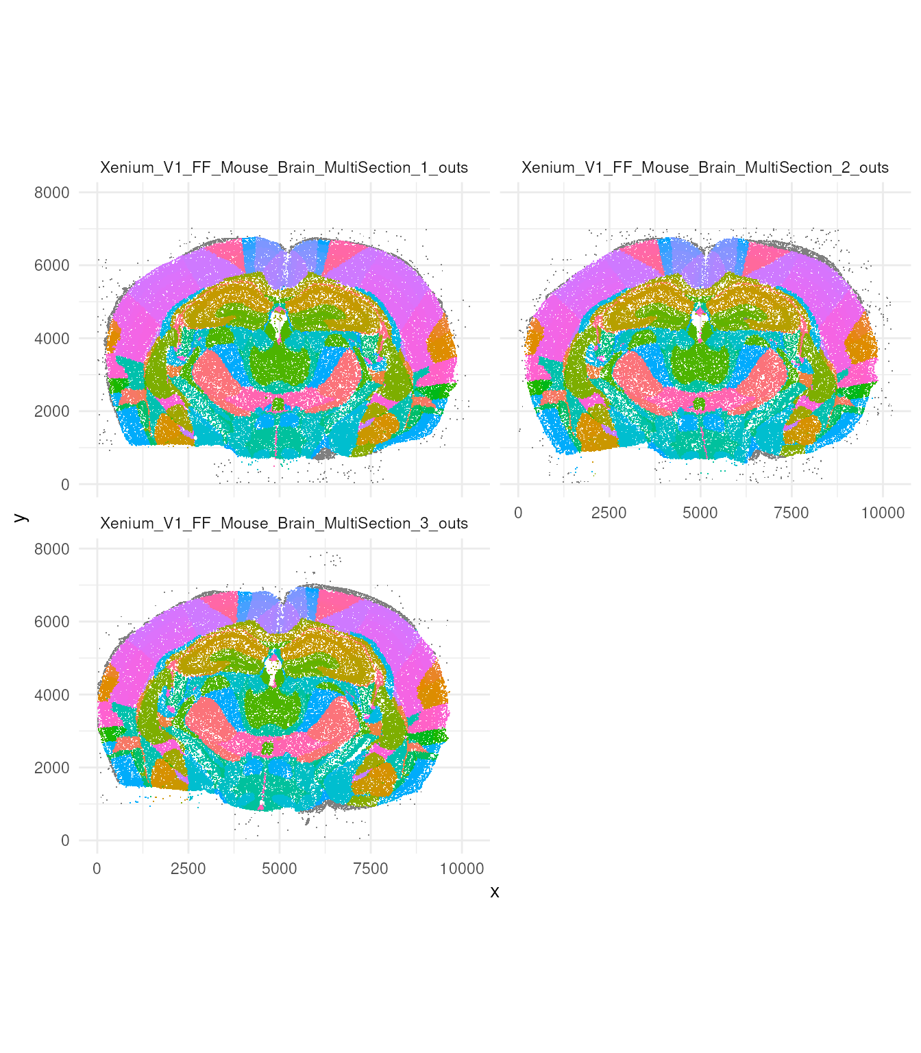
Let’s have a look how many regions have been annotated
tx_small |>
  distinct(region)
## # A tibble: 146 × 1
## region
## <chr>
## 1 NA
## 2 fiber tracts
## 3 LZ
## 4 TEa5
## 5 CTXsp
## 6 VPM
## 7 SSp-bfd5
## 8 cc
## 9 ENTl5
## 10 SSp
## # ℹ 136 more rowsFrom this large dataset, we select a small reagion for illustrative purposes.
If you do not have tx loaded from before, load the pre-saved data:
tx_small_region_file = tempfile()
utils::download.file(
  "https://zenodo.org/records/11213155/files/tx_small_region.rda?download=1",
  destfile = tx_small_region_file,
  mode = "wb"
)
tryCatch(
  load(tx_small_region_file),
  error = function(e) {
    message("Falling back to bundled tx_small_region data: ", conditionMessage(e))
    data("tx_small_region", package = "tidySpatialWorkshop")
  }
)
2. MoleculeExperiment
The R package MoleculeExperiment includes functions to create and manipulate objects from the newly introduced MoleculeExperiment class, designed for analysing molecule-based spatial transcriptomics data from platforms such as Xenium by 10X, CosMx SMI by Nanostring, and Merscope by Vizgen, among others.
MoleculeExperiment class uses cell boundary information
instead of cell identifiers. And thus we won’t use
MoleculeExperiment directly. However, as it is an important
part of bioconductor we briefly introduce this package.
We show how we would import our table of probe location into a
MoleculeExperiment. For this section, we will go through
the example code given in the vignette
material.
library(MoleculeExperiment)

repoDir = system.file("extdata", package = "MoleculeExperiment")
repoDir = paste0(repoDir, "/xenium_V1_FF_Mouse_Brain")

me = readXenium(repoDir, keepCols = "essential")
me
## MoleculeExperiment class
##
## molecules slot (1): detected
## - detected:
## samples (2): sample1 sample2
## -- sample1:
## ---- features (137): 2010300C02Rik Acsbg1 ... Zfp536 Zfpm2
## ---- molecules (962)
## ---- location range: [4900,4919.98] x [6400.02,6420]
## -- sample2:
## ---- features (143): 2010300C02Rik Acsbg1 ... Zfp536 Zfpm2
## ---- molecules (777)
## ---- location range: [4900.01,4919.98] x [6400.16,6419.97]
##
##
## boundaries slot (1): cell
## - cell:
## samples (2): sample1 sample2
## -- sample1:
## ---- segments (5): 67500 67512 67515 67521 67527
## -- sample2:
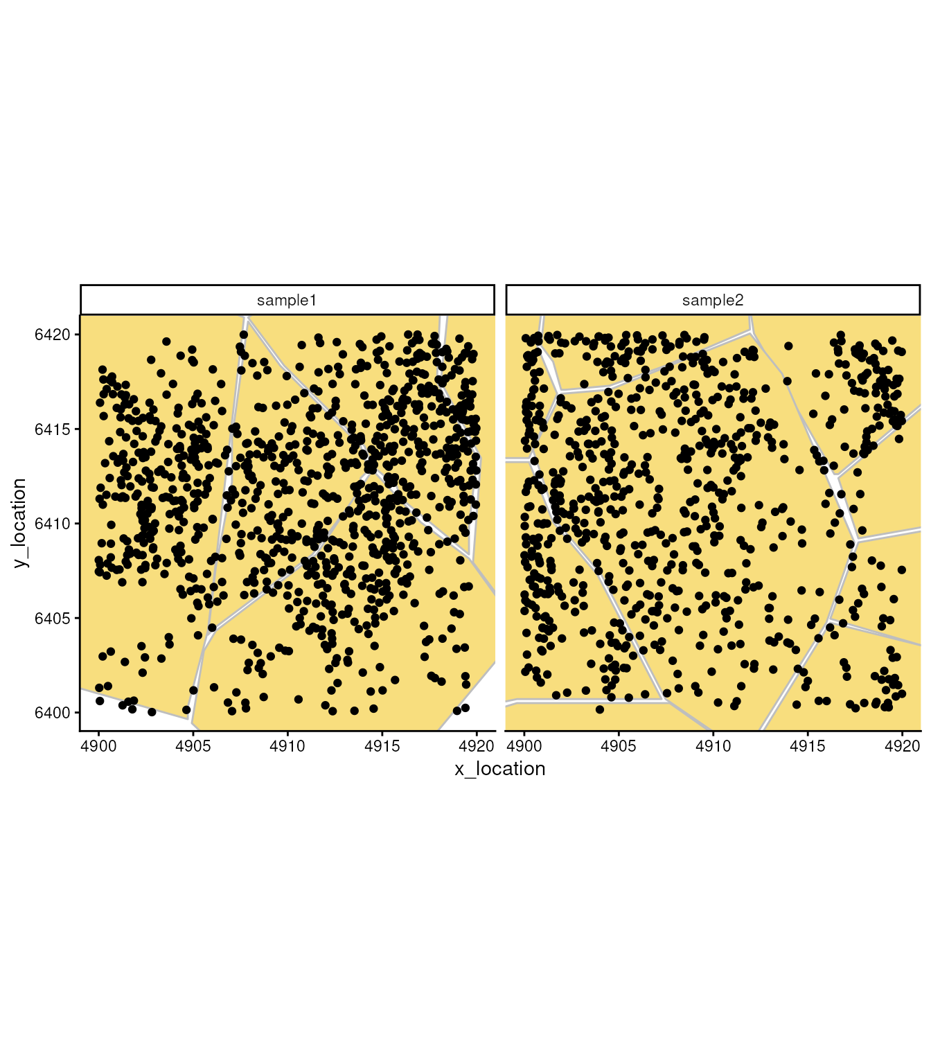
## ---- segments (9): 65043 65044 ... 65070 65071In this object, besides the single molecule location, we have cell segmentation boundaries. We can use these boundaries to understand subcellular localisation of molecules and to aggregate molecules in cells.
ggplot_me() +
  geom_polygon_me(me, assayName = "cell", fill = "#F8DE7E", color="grey") +
  geom_point_me(me) +
  # zoom in to selected patch area
  coord_cartesian(
    xlim = c(4900, 4919.98),
    ylim = c(6400.02, 6420)
  )
In this object we don’t only have the cell segmentation but the nucleus segmentation as well.
boundaries(me, "nucleus") = readBoundaries(
  dataDir = repoDir,
  pattern = "nucleus_boundaries.csv",
  segmentIDCol = "cell_id",
  xCol = "vertex_x",
  yCol = "vertex_y",
  keepCols = "essential",
  boundariesAssay = "nucleus",
  scaleFactorVector = 1
)

boundaries(me, "cell")
## $cell
## $cell$sample1
## $cell$sample1$`67500`
## # A tibble: 13 × 2
## x_location y_location
## <dbl> <dbl>
## 1 4905. 6400.
## 2 4899. 6401.
## 3 4894. 6408.
## 4 4890. 6418.
## 5 4887. 6423.
## 6 4887. 6425.
## 7 4890. 6427.
## 8 4891. 6427.
## 9 4894. 6426.
## 10 4908. 6421.
## 11 4906. 6404.
## 12 4905. 6400.
## 13 4905. 6400.
##
## $cell$sample1$`67512`
## # A tibble: 13 × 2
## x_location y_location
## <dbl> <dbl>
## 1 4906. 6404.
## 2 4906. 6408.
## 3 4907. 6412.
## 4 4907. 6415.
## 5 4908. 6421.
## 6 4910. 6418.
## 7 4914. 6414.
## 8 4914. 6413.
## 9 4914. 6412.
## 10 4914. 6412.
## 11 4911. 6408.
## 12 4906. 6405.
## 13 4906. 6404.
##
## $cell$sample1$`67515`
## # A tibble: 13 × 2
## x_location y_location
## <dbl> <dbl>
## 1 4909. 6396.
## 2 4905. 6399.
## 3 4906. 6403.
## 4 4906. 6404.
## 5 4912. 6408.
## 6 4914. 6413.
## 7 4917. 6410.
## 8 4920. 6408.
## 9 4922. 6404.
## 10 4916. 6397.
## 11 4913. 6396.
## 12 4910. 6396.
## 13 4909. 6396.
##
## $cell$sample1$`67521`
## # A tibble: 13 × 2
## x_location y_location
## <dbl> <dbl>
## 1 4920. 6408.
## 2 4916. 6411.
## 3 4916. 6412.
## 4 4914. 6413.
## 5 4914. 6414.
## 6 4910. 6418.
## 7 4908. 6421.
## 8 4919. 6428.
## 9 4918. 6422.
## 10 4918. 6418.
## 11 4920. 6413.
## 12 4920. 6410.
## 13 4920. 6408.
##
## $cell$sample1$`67527`
## # A tibble: 13 × 2
## x_location y_location
## <dbl> <dbl>
## 1 4922. 6405.
## 2 4920. 6408.
## 3 4920. 6413.
## 4 4918. 6418.
## 5 4919. 6428.
## 6 4922. 6432.
## 7 4927. 6430.
## 8 4927. 6414.
## 9 4929. 6409.
## 10 4929. 6408.
## 11 4928. 6408.
## 12 4923. 6405.
## 13 4922. 6405.
##
##
## $cell$sample2
## $cell$sample2$`65043`
## # A tibble: 13 × 2
## x_location y_location
## <dbl> <dbl>
## 1 4897. 6413.
## 2 4895. 6414.
## 3 4894. 6418.
## 4 4892. 6421.
## 5 4886. 6423.
## 6 4888. 6426.
## 7 4897. 6430.
## 8 4904. 6429.
## 9 4901. 6425.
## 10 4901. 6419.
## 11 4902. 6417.
## 12 4900. 6413.
## 13 4897. 6413.
##
## $cell$sample2$`65044`
## # A tibble: 13 × 2
## x_location y_location
## <dbl> <dbl>
## 1 4902. 6417.
## 2 4902. 6419.
## 3 4901. 6419.
## 4 4901. 6423.
## 5 4902. 6425.
## 6 4905. 6429.
## 7 4910. 6431.
## 8 4912. 6424.
## 9 4912. 6420.
## 10 4907. 6418.
## 11 4904. 6417.
## 12 4902. 6417.
## 13 4902. 6417.
##
## $cell$sample2$`65051`
## # A tibble: 13 × 2
## x_location y_location
## <dbl> <dbl>
## 1 4916. 6413.
## 2 4912. 6420.
## 3 4910. 6431.
## 4 4914. 6439.
## 5 4919. 6444.
## 6 4924. 6443.
## 7 4928. 6442.
## 8 4934. 6437.
## 9 4938. 6429.
## 10 4939. 6424.
## 11 4922. 6417.
## 12 4917. 6413.
## 13 4916. 6413.
##
## $cell$sample2$`65055`
## # A tibble: 13 × 2
## x_location y_location
## <dbl> <dbl>
## 1 4912. 6398.
## 2 4907. 6401.
## 3 4904. 6407.
## 4 4902. 6410.
## 5 4900. 6414.
## 6 4902. 6417.
## 7 4904. 6417.
## 8 4912. 6420.
## 9 4914. 6418.
## 10 4917. 6409
## 11 4916. 6405.
## 12 4912. 6398.
## 13 4912. 6398.
##
## $cell$sample2$`65063`
## # A tibble: 13 × 2
## x_location y_location
## <dbl> <dbl>
## 1 4930. 6408.
## 2 4925. 6410.
## 3 4921. 6410.
## 4 4918. 6409.
## 5 4917. 6412.
## 6 4922. 6417.
## 7 4927. 6419.
## 8 4931. 6421.
## 9 4939. 6423.
## 10 4939. 6423.
## 11 4938. 6422.
## 12 4930. 6408.
## 13 4930. 6408.
##
## $cell$sample2$`65064`
## # A tibble: 13 × 2
## x_location y_location
## <dbl> <dbl>
## 1 4891. 6399.
## 2 4888. 6400.
## 3 4888. 6410.
## 4 4892. 6411.
## 5 4895. 6414.
## 6 4897. 6413.
## 7 4900. 6413.
## 8 4902. 6410.
## 9 4904. 6407.
## 10 4907. 6401.
## 11 4900. 6401.
## 12 4893. 6399.
## 13 4891. 6399.
##
## $cell$sample2$`65067`
## # A tibble: 13 × 2
## x_location y_location
## <dbl> <dbl>
## 1 4925. 6403.
## 2 4924. 6403.
## 3 4922. 6403.
## 4 4921. 6403.
## 5 4916. 6405.
## 6 4918. 6409
## 7 4921. 6410.
## 8 4925. 6410.
## 9 4927. 6409.
## 10 4930. 6408.
## 11 4930. 6408.
## 12 4925. 6403.
## 13 4925. 6403.
##
## $cell$sample2$`65070`
## # A tibble: 13 × 2
## x_location y_location
## <dbl> <dbl>
## 1 4901. 6389.
## 2 4899. 6391.
## 3 4899. 6392.
## 4 4896. 6395.
## 5 4892. 6399.
## 6 4897. 6400.
## 7 4900. 6400.
## 8 4908. 6400.
## 9 4911. 6398.
## 10 4912. 6397.
## 11 4909. 6390.
## 12 4902. 6389.
## 13 4901. 6389.
##
## $cell$sample2$`65071`
## # A tibble: 13 × 2
## x_location y_location
## <dbl> <dbl>
## 1 4924. 6394.
## 2 4922. 6395.
## 3 4917. 6396.
## 4 4912. 6397.
## 5 4912. 6398.
## 6 4916. 6405.
## 7 4922. 6403.
## 8 4923. 6403.
## 9 4925. 6402.
## 10 4925. 6401.
## 11 4925. 6400.
## 12 4925. 6394.
## 13 4924. 6394.
showMolecules(me)## List of 1
## $ detected:List of 2
## ..$ sample1:List of 137
## .. ..$ 2010300C02Rik : tibble [11 × 2] (S3: tbl_df/tbl/data.frame)
## .. ..$ Acsbg1 : tibble [6 × 2] (S3: tbl_df/tbl/data.frame)
## .. .. [list output truncated]
## ..$ sample2:List of 143
## .. ..$ 2010300C02Rik: tibble [9 × 2] (S3: tbl_df/tbl/data.frame)
## .. ..$ Acsbg1 : tibble [10 × 2] (S3: tbl_df/tbl/data.frame)
## .. .. [list output truncated]
bds_colours = setNames(
  c("#aa0000ff", "#ffaaffff"),
  c("Region 1", "Region 2")
)

ggplot_me() +
  # add cell segments and colour by cell id
  geom_polygon_me(me, byFill = "segment_id", colour = "black", alpha = 0.1) +
  # add molecule points and colour by feature name
  geom_point_me(me, byColour = "feature_id", size = 0.1) +
  # add nuclei segments and colour the border with red
  geom_polygon_me(me, assayName = "nucleus", fill = NA, colour = "red") +
  # zoom in to selected patch area
  coord_cartesian(xlim = c(4900, 4919.98), ylim = c(6400.02, 6420))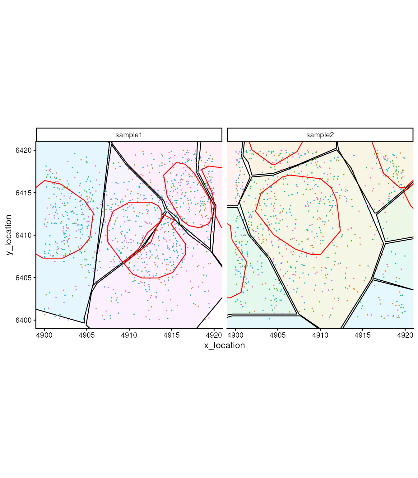
##            used  (Mb) gc trigger   (Mb) max used  (Mb)
## Ncells 11301643 603.6   20123925 1074.8 15425935 823.9
## Vcells 45298102 345.6   66994829  511.2 55759668 425.5
MoleculeExperiment also has functions such as
dataframeToMEList() and then
MoleculeExperiment() where we can organise our large data
frame containing single molecules into a more efficient
MoleculeExperiment object.
library(MoleculeExperiment)

tx_small_me =
  tx_small |>
    select(sample_id, gene, x, y) |>
    dataframeToMEList(
        dfType = "molecules",
        assayName = "detected",
        sampleCol = "sample_id",
        factorCol = "gene",
        xCol = "x",
        yCol = "y"
    ) |>
    MoleculeExperiment()

tx_small_me
## MoleculeExperiment class
##
## molecules slot (1): detected
## - detected:
## samples (3): Xenium_V1_FF_Mouse_Brain_MultiSection_1_outs
## Xenium_V1_FF_Mouse_Brain_MultiSection_2_outs
## Xenium_V1_FF_Mouse_Brain_MultiSection_3_outs
## -- Xenium_V1_FF_Mouse_Brain_MultiSection_1_outs:
## ---- features (496): 2010300C02Rik Acsbg1 ... Zfp536 Zfpm2
## ---- molecules (125531)
## ---- location range: [20,10197.56] x [31.25,7021.59]
## -- Xenium_V1_FF_Mouse_Brain_MultiSection_2_outs:
## ---- features (483): 2010300C02Rik Acsbg1 ... Zfp536 Zfpm2
## ---- molecules (116929)
## ---- location range: [28.65,10256.49] x [43.5,7012.21]
## -- Xenium_V1_FF_Mouse_Brain_MultiSection_3_outs:
## ---- features (488): 2010300C02Rik Acsbg1 ... Zfp536 Zfpm2
## ---- molecules (119310)
## ---- location range: [10.6,9656.13] x [45.85,7884.78]
##
##
## boundaries slot: NULLHere, we can appreciate the difference in size between the redundant data frame
tx_small |>
  object.size() |>
  format(units = "auto")
## [1] "69.1 Mb"and the MoleculeExperiment.
tx_small_me |>
  object.size() |>
  format(units = "auto")
## [1] "7 Mb"## used (Mb) gc trigger (Mb) max used (Mb)
## Ncells 11303581 603.7 20123925 1074.8 15425935 823.9
## Vcells 36258616 276.7 66994829 511.2 64531492 492.4A preview of a zoomed in section of the tissue
Now let’s try to visualise just a small section,
tx_small_region, that we downloaded earlier. You can
appreciate, single molecules are coloured by cell. You can also
appreciate the difference in density between regions. An aspect to note,
is that not all probes are within cells. This depends on the
segmentation process.
brewer.pal(7, "Set1")## [1] "#E41A1C" "#377EB8" "#4DAF4A" "#984EA3" "#FF7F00" "#FFFF33" "#A65628"
tx_small_region |>
  filter(!is.na(cell)) |>
  slice_sample(prop = 0.3) |>
  ggplot(aes(x, y, colour = factor(cell))) +
  geom_point(shape=".") +

  facet_wrap(~sample_id, ncol = 2) +
  scale_color_manual(values = sample(colorRampPalette(brewer.pal(8, "Set2"))(1800))) +
  coord_fixed() +
  theme_minimal() +
  theme(legend.position = "none")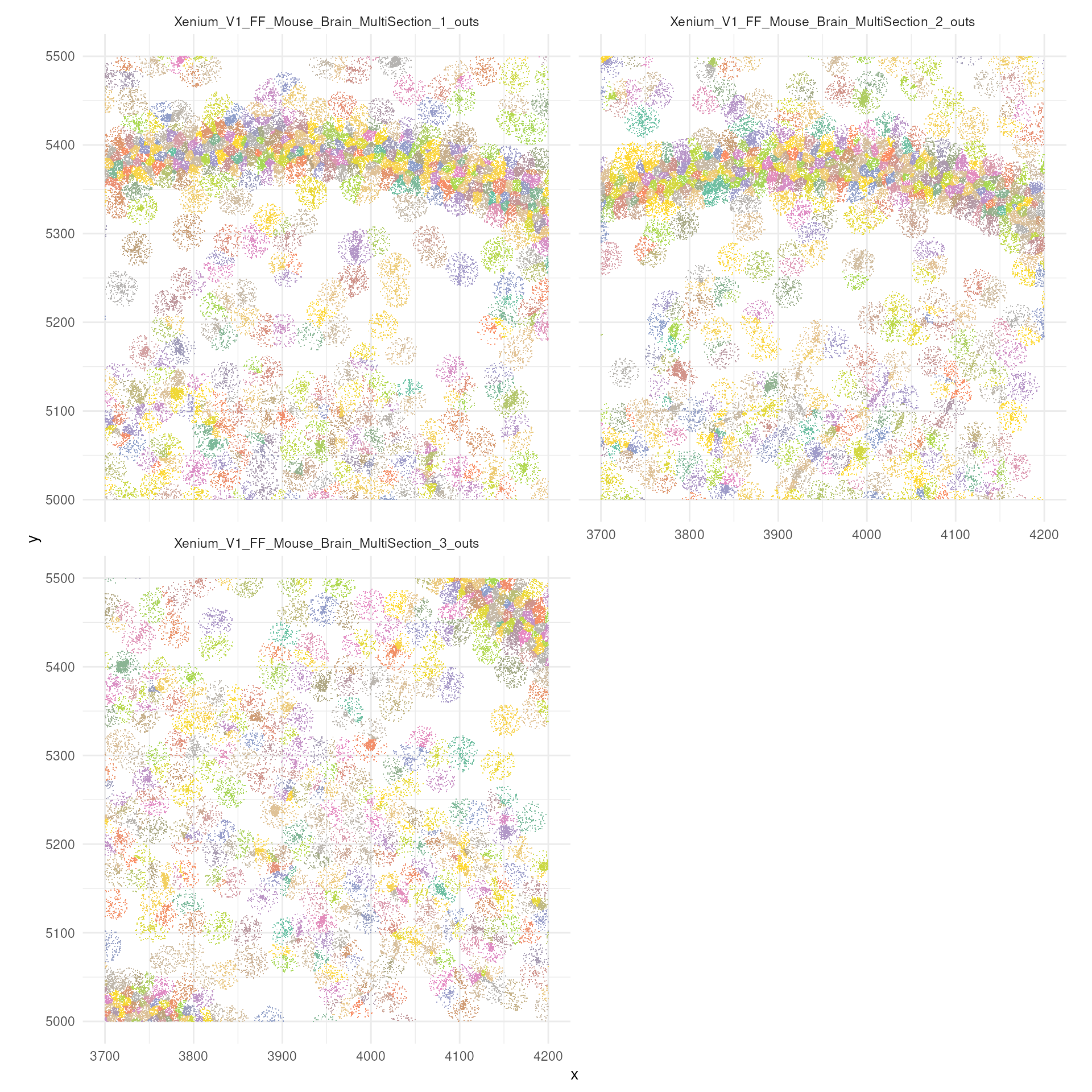
Let’s have a look to the probes that have not being unassigned to cells.
tx_small_region |>
  filter(is.na(cell)) |>
  ggplot(aes(x, y, colour = factor(cell))) +
  geom_point(shape=".") +
  facet_wrap(~sample_id, ncol = 2) +
  scale_color_manual(values = sample(colorRampPalette(brewer.pal(8, "Set2"))(1800))) +
  coord_fixed() +
  theme_minimal() +
  theme(legend.position = "none")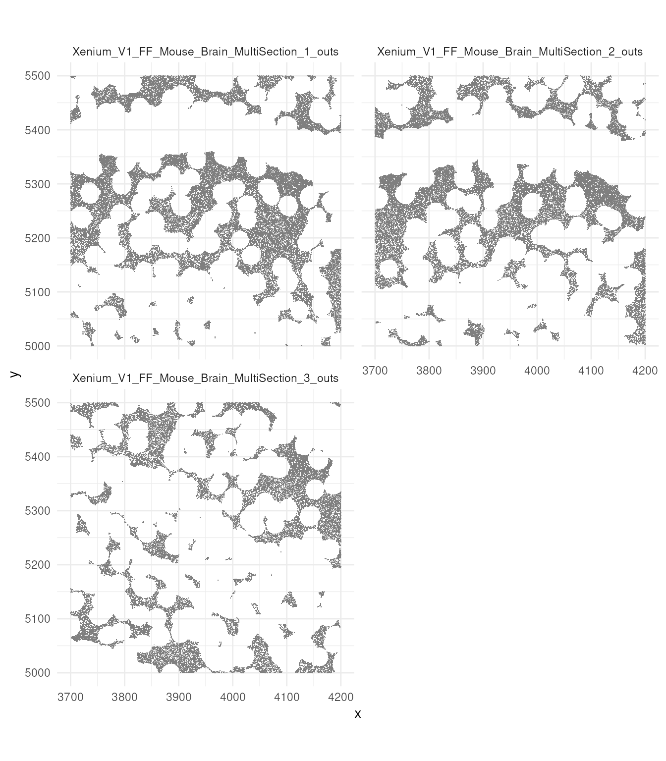
Exercise 3.1
We want to understand how much data we are discarding, that does not have a cell identity.
- Using base R grammar calculate what is the ratio of outside-cell vs within-cell, probes
- Reproduce the same calculation with
tidyverse - Calculate the percentage of probes are within the cytoplasm but outside the nucleus
##            used (Mb) gc trigger   (Mb) max used  (Mb)
## Ncells 11327338  605   20123925 1074.8 15425935 823.9
## Vcells 21493359  164   66994829  511.2 66989641 511.1
3. Aggregation and analysis
We will convert our cell by gene count to a
SpatialExperiment. This object stores a cell by gene matrix
with relative XY coordinates.
SubcellularSpatialData package has a utility function
that aggregated the single molecules in cells, where these cell ID have
been identified with segmentation.
If you do not have tx loaded from before, load the pre-saved data
converted to SpatialExperiment:
tx_spe_file = tempfile()
utils::download.file(
  "https://zenodo.org/records/11213166/files/tx_spe.rda?download=1",
  destfile = tx_spe_file,
  mode = "wb"
)
# load("~/Downloads/tx_spe.rda")
load(tx_spe_file)
Keep just the annotated regions.
## Warning: `when()` was deprecated in purrr 1.0.0.
## ℹ Please use `if` instead.
## ℹ The deprecated feature was likely used in the tidySpatialExperiment package.
##   Please report the issue at
##   <https://github.com/william-hutchison/tidySpatialExperiment/issues>.
## This warning is displayed once per session.
## Call `lifecycle::last_lifecycle_warnings()` to see where this warning was
## generated.
Let have a look to the SpatialExperiment.
tx_spe## # A SpatialExperiment-tibble abstraction: 467,131 × 8
## # Features = 541 | Cells = 467131 | Assays = counts
## .cell sample_id cell_id transcript_id qv region x y
## <chr> <fct> <fct> <dbl> <dbl> <fct> <dbl> <dbl>
## 1 Xenium_V1_FF_Mouse_… 1 1 2.82e14 31.4 CP 1557. 2529.
## 2 Xenium_V1_FF_Mouse_… 1 10 2.82e14 32.2 CP 1631. 2543.
## 3 Xenium_V1_FF_Mouse_… 1 100 2.82e14 30.7 Isoco… 834. 3109.
## 4 Xenium_V1_FF_Mouse_… 1 1000 2.82e14 31.4 RSPv5 4932. 5720.
## 5 Xenium_V1_FF_Mouse_… 1 10000 2.82e14 31.5 LA 1667. 2159.
## 6 Xenium_V1_FF_Mouse_… 1 100000 2.82e14 33.6 VISa1 3558. 6587.
## 7 Xenium_V1_FF_Mouse_… 1 100001 2.82e14 31.7 VISa1 3570. 6583.
## 8 Xenium_V1_FF_Mouse_… 1 100002 2.82e14 33.9 SSp 3430. 6157.
## 9 Xenium_V1_FF_Mouse_… 1 100003 2.82e14 32.5 SSp 3431. 6120.
## 10 Xenium_V1_FF_Mouse_… 1 100004 2.82e14 33.5 SSp 3436. 6140.
## # ℹ 467,121 more rowsHere we introduce the ggspavis package to visualize
spatial transcriptomics data. This package requires a column called
in_tissue to be present in the
SpatialExperiment object. Here we edit our data include
this column.
tx_spe = tx_spe |> mutate(in_tissue = TRUE) Let’s have a look to our SpatialExperiment.
tx_spe## # A SpatialExperiment-tibble abstraction: 467,131 × 9
## # Features = 541 | Cells = 467131 | Assays = counts
## .cell sample_id cell_id transcript_id qv region in_tissue x y
## <chr> <fct> <fct> <dbl> <dbl> <fct> <lgl> <dbl> <dbl>
## 1 Xenium_V1… 1 1 2.82e14 31.4 CP TRUE 1557. 2529.
## 2 Xenium_V1… 1 10 2.82e14 32.2 CP TRUE 1631. 2543.
## 3 Xenium_V1… 1 100 2.82e14 30.7 Isoco… TRUE 834. 3109.
## 4 Xenium_V1… 1 1000 2.82e14 31.4 RSPv5 TRUE 4932. 5720.
## 5 Xenium_V1… 1 10000 2.82e14 31.5 LA TRUE 1667. 2159.
## 6 Xenium_V1… 1 100000 2.82e14 33.6 VISa1 TRUE 3558. 6587.
## 7 Xenium_V1… 1 100001 2.82e14 31.7 VISa1 TRUE 3570. 6583.
## 8 Xenium_V1… 1 100002 2.82e14 33.9 SSp TRUE 3430. 6157.
## 9 Xenium_V1… 1 100003 2.82e14 32.5 SSp TRUE 3431. 6120.
## 10 Xenium_V1… 1 100004 2.82e14 33.5 SSp TRUE 3436. 6140.
## # ℹ 467,121 more rowsLet’s have a look at how many cells have been detected for each region
tx_spe |>
  add_count(region) |>
  ggplot(aes(fct_reorder(region, n, .desc = TRUE))) +
  geom_bar() +
  theme_bw() +
  theme(axis.text.x  = element_text(angle=90, hjust=1, size = 2))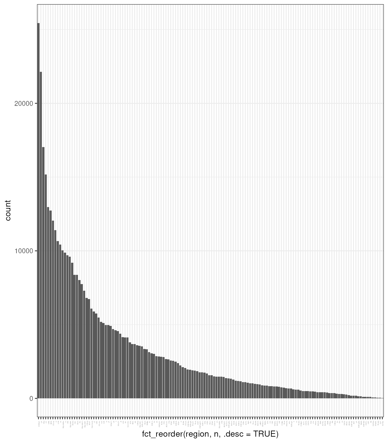
We normalise the SpatialExperiment using
scater.
tx_spe =
  tx_spe |>

  # Scaling and tranformation
  scater::logNormCounts()
## Warning in .library_size_factors(assay(x, assay.type), ...): 'librarySizeFactors' is deprecated.
## Use 'scrapper::centerSizeFactors' instead.
## See help("Deprecated")## Warning in .local(x, ...): 'normalizeCounts' is deprecated.
## Use 'scrapper::normalizeCounts' instead.
## See help("Deprecated")We then visualise what is the relationship between variance and total expression across cells.
tx_spe |>

  # Gene variance
  scran::modelGeneVar(block = tx_spe$sample_id) |>

  # Reformat for plotting
  as_tibble(rownames  = "feature") |>

  # Plot
  ggplot(aes(mean, total)) +
  geom_point() +
  geom_smooth(color="red")+
  xlab("Mean log-expression") +
  ylab("Variance") +
  theme_bw()
## Warning in fitTrendVar(fm, fv, ...): 'fitTrendVar' is deprecated.
## Use 'scrapper::fitVarianceTrend' instead.
## See help("Deprecated")
## Warning in fitTrendVar(fm, fv, ...): 'fitTrendVar' is deprecated.
## Use 'scrapper::fitVarianceTrend' instead.
## See help("Deprecated")
## Warning in fitTrendVar(fm, fv, ...): 'fitTrendVar' is deprecated.
## Use 'scrapper::fitVarianceTrend' instead.
## See help("Deprecated")## Warning in combineBlocks(collected, method = method, equiweight = equiweight, : 'combineBlocks' is deprecated.
## See help("Deprecated")## `geom_smooth()` using method = 'loess' and formula = 'y ~ x'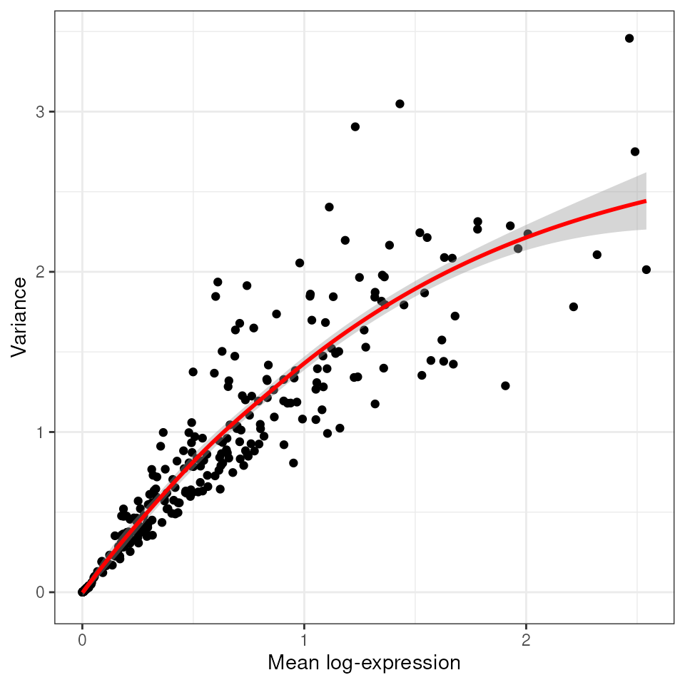
For further analysis, we subset the dataset to allow quicker calculations.
tx_spe_sample_1 =
  tx_spe |>
  filter(sample_id=="1") |>
  slice_sample(prop = 0.2)
As we have done previously, we calculate variable informative genes, for further analyses.
genes <- !grepl(pattern = "NegControl.+|BLANK.+", x = rownames(tx_spe_sample_1))

# Get the top 2000 genes.
top.hvgs =
  tx_spe_sample_1 |>

  scran::modelGeneVar(subset.row = genes) |>

  # Model gene variance and select variable genes per sample
  getTopHVGs(n=200)
## Warning in getTopHVGs(scran::modelGeneVar(tx_spe_sample_1, subset.row = genes), : 'getTopHVGs' is deprecated.
## Use 'scrapper::chooseHighlyVariableGenes' instead.
## See help("Deprecated")## Warning in fitTrendVar(fm, fv, ...): 'fitTrendVar' is deprecated.
## Use 'scrapper::fitVarianceTrend' instead.
## See help("Deprecated")## Warning in combineBlocks(collected, method = method, equiweight = equiweight, : 'combineBlocks' is deprecated.
## See help("Deprecated")
top.hvgs## [1] "Gjc3" "Gfap" "Opalin" "Igf2"
## [5] "Slc17a6" "Slc17a7" "Sox10" "Neurod6"
## [9] "Calb2" "Ly6a" "Cldn5" "Gad1"
## [13] "Fn1" "Gad2" "Lamp5" "Penk"
## [17] "Pdgfra" "Cabp7" "Prox1" "Dcn"
## [21] "Nr2f2" "Aqp4" "Pvalb" "Arc"
## [25] "Laptm5" "Adgrl4" "Slc13a4" "Rims3"
## [29] "Vat1l" "Calb1" "Bhlhe22" "Cspg4"
## [33] "Pecam1" "Nwd2" "Dkk3" "Meis2"
## [37] "Gpr17" "Aldh1a2" "Necab1" "Cd24a"
## [41] "Epha4" "Rprm" "Car4" "Nrn1"
## [45] "Siglech" "Ccn2" "Acta2" "Fmod"
## [49] "Kdr" "Ntsr2" "Spp1" "Acsbg1"
## [53] "2010300C02Rik" "Trem2" "Igfbp4" "Tmem163"
## [57] "Col1a1" "Satb2" "Col6a1" "Spag16"
## [61] "Rab3b" "Nxph3" "Slc39a12" "Cd53"
## [65] "Emcn" "Acvrl1" "Rasgrf2" "Nts"
## [69] "Cplx3" "Gjb2" "Hs3st2" "Cd93"
## [73] "Cbln4" "Plcxd3" "Bcl11b" "Pdyn"
## [77] "Carmn" "Syt6" "Cpne4" "Foxp2"
## [81] "Fezf2" "Clmn" "Cobll1" "Myl4"
## [85] "Sox17" "Cyp1b1" "Sncg" "Bdnf"
## [89] "Necab2" "Sst" "Nell1" "Paqr5"
## [93] "Pln" "Cpne6" "Unc13c" "Pglyrp1"
## [97] "Vip" "Cbln1" "Rnf152" "Ebf3"
## [101] "Ano1" "Hapln1" "Igfbp6" "Sema3d"
## [105] "Sema3e" "Zfp536" "Rmst" "Cdh13"
## [109] "Tmem255a" "Cd300c2" "Adamtsl1" "Ikzf1"
## [113] "Pou3f1" "Crh" "Prdm8" "Rxfp1"The selected subset of genes can then be passed to the subset.row argument (or equivalent) in downstream steps.
tx_spe_sample_1 =
  tx_spe_sample_1 |>

  # We use fixed PCA as we have a limited number of features
  fixedPCA( subset.row=top.hvgs )
## Warning in fixedPCA(tx_spe_sample_1, subset.row = top.hvgs): 'fixedPCA' is deprecated.
## Use 'scrapper::runPca.se' instead.
## See help("Deprecated")We then use the gene expression to cluster sales based on their similarity and represent these clusters in a two dimensional embeddings (UMAP)
Louvain clustering is a popular method used in single-cell RNA sequencing (scRNA-seq) data analysis to identify groups of cells with similar gene expression profiles. This method is based on the Louvain algorithm, which is widely used for detecting community structures in large networks.
The Louvain algorithm is designed to maximize a metric known as modularity, which measures the density of edges inside communities compared to edges outside communities.
It operates in two phases:
- first, it looks for small communities by optimizing modularity locally, and
- second it aggregates nodes belonging to the same community and repeats the process.
cluster_labels =
  tx_spe_sample_1 |>
   scran::clusterCells(
     use.dimred="PCA",
     BLUSPARAM=bluster::NNGraphParam(k=30, cluster.fun="louvain")
    ) |>
   as.character()
## Warning in scran::clusterCells(tx_spe_sample_1, use.dimred = "PCA", BLUSPARAM = bluster::NNGraphParam(k = 30, : 'clusterCells' is deprecated.
## Use 'bluster::clusterRows' instead.
## See help("Deprecated")
cluster_labels |>
  head()
## [1] "1" "2" "3" "2" "4" "5"Now we add this cluster column to our
SpatialExperiment
tx_spe_sample_1 =
  tx_spe_sample_1 |>
  mutate(my_clusters = cluster_labels)

tx_spe_sample_1 |> select(.cell, my_clusters)
## # A SpatialExperiment-tibble abstraction: 31,938 × 10
## # Features = 541 | Cells = 31938 | Assays = counts, logcounts
## .cell my_clusters sample_id x y PC1 PC2 PC3 PC4 PC5
## <chr> <chr> <fct> <dbl> <dbl> <dbl> <dbl> <dbl> <dbl> <dbl>
## 1 Xenium_V… 1 1 2654. 5443. -2.30 0.426 -4.56 2.59 2.54
## 2 Xenium_V… 2 1 7424. 4891. 7.97 0.783 -5.36 2.46 -0.397
## 3 Xenium_V… 3 1 4546. 6732. 3.84 -5.78 1.65 -2.54 2.63
## 4 Xenium_V… 2 1 2457. 3507. 9.59 -1.23 -3.60 -0.854 4.77
## 5 Xenium_V… 4 1 9549. 2918. -6.51 0.629 -0.224 -1.54 1.67
## 6 Xenium_V… 5 1 4503. 849. 5.80 -1.18 5.03 -0.503 -1.89
## 7 Xenium_V… 6 1 4842. 4963. -5.59 -1.25 -2.43 1.78 1.61
## 8 Xenium_V… 7 1 8846. 4544. -5.09 -3.93 3.33 2.35 2.66
## 9 Xenium_V… 1 1 2550. 5421. -4.75 -1.96 -2.86 -1.23 0.419
## 10 Xenium_V… 2 1 3460. 1581. 8.70 2.90 -4.57 1.56 -0.919
## # ℹ 31,928 more rowsAs we have done before, we caclculate UMAPs for visualisation purposes.
This step takes long time.
## Check how many
tx_spe_sample_1 =
  tx_spe_sample_1 |>
  runUMAP()
Now, let’s visualise the my_clusters in UMAP space.
tx_spe_sample_1 |>
  plotUMAP(colour_by = "my_clusters") +
  scale_color_discrete(
    colorRampPalette(brewer.pal(9, "Set1"))(30)
  )
## Scale for colour is already present.
## Adding another scale for colour, which will replace the existing scale.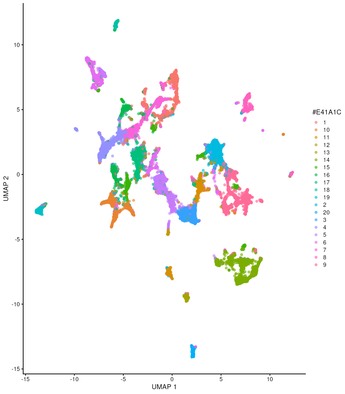
Exercise 3.2
Let’s try to understand the identity of these clusters performing gene marker detection.
In the previous sections we have seen how to do gene marker selection for sequencing-based spatial data. We just have to adapt it to our current scenario.
Score the markers (scran::scoreMarkers or tx_spe_sample_1)
Filter top markers (filter mean.AUC > 0.8)
Focus on Cluster 1 and try to guess the cell type (subset first element in the list, copy and paste the first 5 genes, and quickly look in public resources about what cell type those gene are markers of)
Plot the umap colouring by the top marker of cluster 1 (plotReducedDim())
To understand whether the cell clusters explain morphology as opposed to merely cell identity, we can color cells according to annotated region. As we can see we have a lot of regions. We have more regions that cell clusters.
tx_spe_sample_1 |>
  plotUMAP(colour_by = "region") +
  scale_color_discrete(
    brewer.pal(n = 30, name = "Set1")
  ) +
  guides(color="none")
## Warning in brewer.pal(n = 30, name = "Set1"): n too large, allowed maximum for palette Set1 is 9
## Returning the palette you asked for with that many colors## Scale for colour is already present.
## Adding another scale for colour, which will replace the existing scale.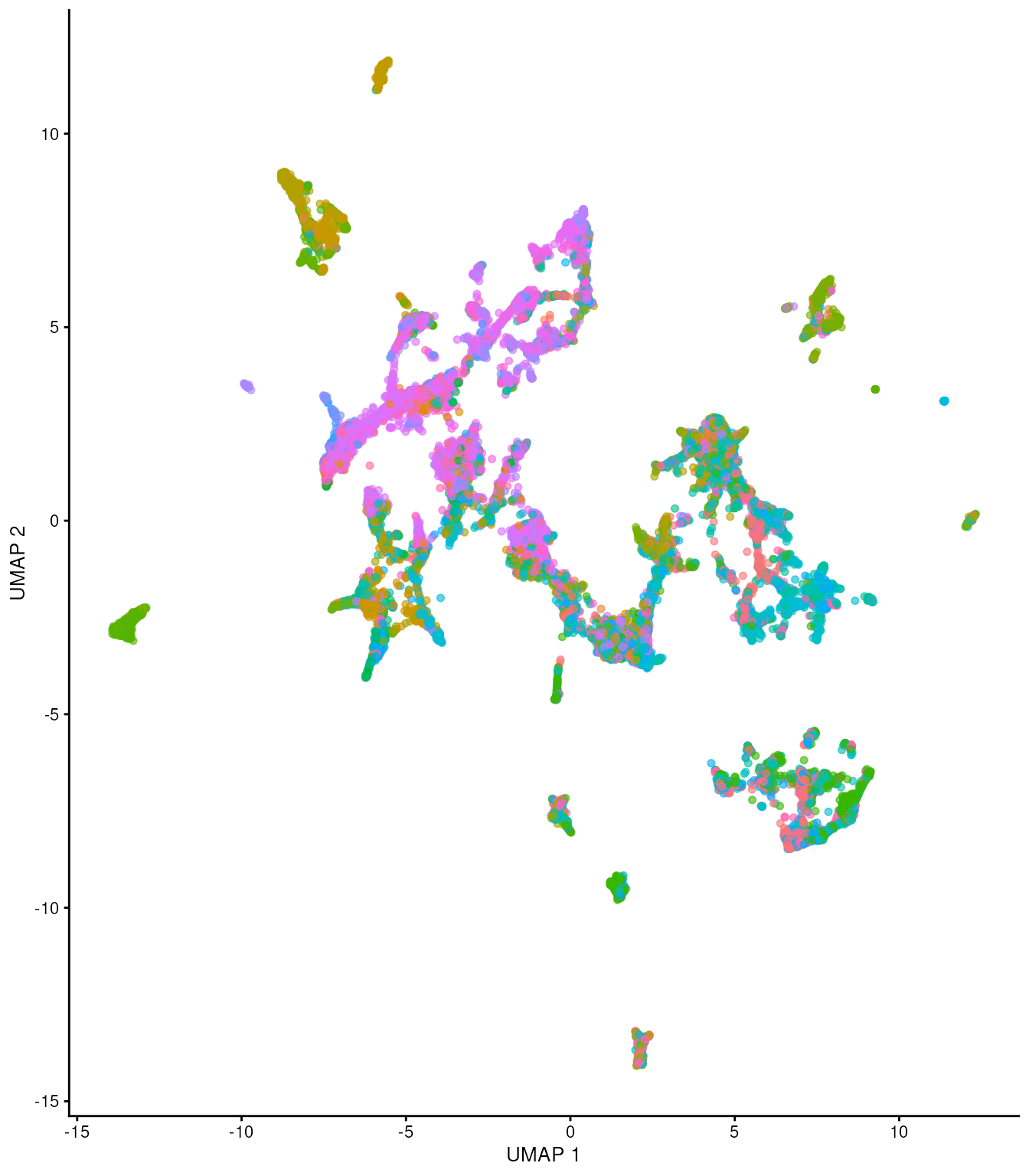
Let’s try to understand the morphological distribution of cell clusters in space.
Plot ground truth in tissue map.
tx_spe_sample_1 |>
  ggspavis::plotCoords(annotate = "my_clusters") +
  guides(color = "none")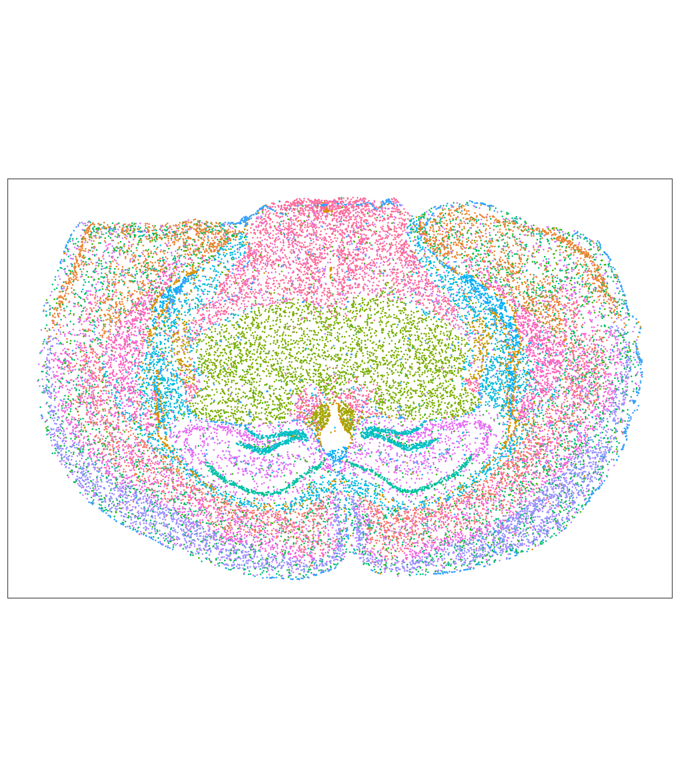
# For comparison the annotated regions (separate chunk so knitr records both figures)
tx_spe_sample_1 |>
  ggspavis::plotCoords(annotate = "region") +
  scale_color_manual(values = colorRampPalette(brewer.pal(9, "Set1"))(150)) +
  guides(color = "none")
## Scale for colour is already present.
## Adding another scale for colour, which will replace the existing scale.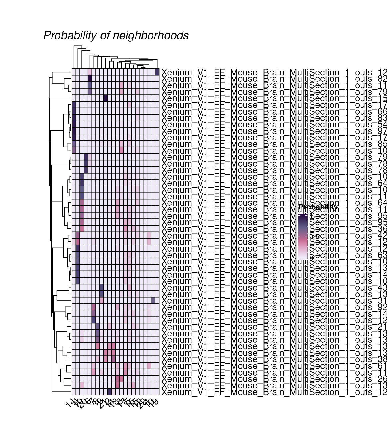
Exercise 3.3
Spatial-aware clustering: Apply the spatial aware clustering method BANKSY. Taking as example the code run for Session 1.
4. Neighborhood analyses
hoodscanR Liu et al., 2025
Algorithm:
Nearest cells detection by Approximate Nearest Neighbor (ANN) search algorithm
Calculating euclidean distance matrix between cells and their k-nearest neighbors
Cell-level annotations provided by users are used to construct a cell annotation matrix
Identify cellular neighborhoods uses the SoftMax function, enhanced by a “shape” parameter that governs the “influence radius”. This measures probability of a cell type to be found in a neighbour.
The K-means clustering algorithm finds recurring neighbours
Before we scan cellular neighborhoods, each cell needs a biological
label rather than an unsupervised cluster ID. We annotate cells with
SingleR, using the human prefrontal cortex reference
prepared in Session 1. Our Xenium panel reports mouse gene symbols,
whereas the Zhong reference uses human symbols; for this workshop we
harmonise identifiers by converting both to upper case so that
orthologous symbols in the panel can be matched. In your own analyses,
use a reference matched to the species and tissue under study.
library(scRNAseq)
library(SingleR)

# Get reference (same workflow as Session 1)
brain_reference <- fetchDataset("zhong-prefrontal-2018", "2023-12-22")

brain_reference =
  brain_reference |>
  scuttle::aggregateAcrossCells(ids = paste(brain_reference$sample, brain_reference$cell_types, sep = "_"))

brain_reference = brain_reference[, brain_reference |> assay() |> colSums() > 0]
brain_reference = brain_reference[, !brain_reference$cell_types |> is.na()]

brain_reference =
  brain_reference |>
  logNormCounts()
Prepare the imaging data for annotation, as we did for the spatial data in Session 1.
tx_spe_sample_1_annot =
  tx_spe_sample_1[
    !grepl("NegControl.+|BLANK.+", rownames(tx_spe_sample_1)),
  ]
rownames(tx_spe_sample_1_annot) <- toupper(rownames(tx_spe_sample_1_annot))
tx_spe_sample_1_annot <- logNormCounts(tx_spe_sample_1_annot)

rownames(brain_reference) <- toupper(rownames(brain_reference))

genes_for_annotation <-
  grep("(^MT-)|(^mt-)|(\\.)|(-)", rownames(brain_reference), value = TRUE, invert = TRUE) |>
  intersect(rownames(tx_spe_sample_1_annot))
We can now annotate each cell with SingleR. With a
targeted Xenium panel we only use genes present in both datasets
(genes_for_annotation). In SingleR, the
genes argument does not take a character
vector of gene names: it must be "de" (automatic marker
detection within the reference) or a named list of
markers per cell type. To limit analysis to the panel, pass those genes
via row subsetting and/or restrict.
singler_pred <- SingleR(
  test = tx_spe_sample_1_annot[genes_for_annotation, ],
  ref = brain_reference[genes_for_annotation, ],
  labels = brain_reference$cell_types,
  genes = "de",
  de.method = "wilcox",
  hint.sce = FALSE
)
tx_spe_sample_1 =
  tx_spe_sample_1 |>
  mutate(cell_type = singler_pred$labels)

tx_spe_sample_1 |> select(.cell, my_clusters, cell_type)
## # A SpatialExperiment-tibble abstraction: 31,938 × 13
## # Features = 541 | Cells = 31938 | Assays = counts, logcounts
## .cell my_clusters cell_type sample_id x y PC1 PC2 PC3 PC4
## <chr> <chr> <chr> <fct> <dbl> <dbl> <dbl> <dbl> <dbl> <dbl>
## 1 Xeniu… 1 OPC 1 2654. 5443. -2.30 0.426 -4.56 2.59
## 2 Xeniu… 2 Astrocyt… 1 7424. 4891. 7.97 0.783 -5.36 2.46
## 3 Xeniu… 3 Microglia 1 4546. 6732. 3.84 -5.78 1.65 -2.54
## 4 Xeniu… 2 OPC 1 2457. 3507. 9.59 -1.23 -3.60 -0.854
## 5 Xeniu… 4 Neurons 1 9549. 2918. -6.51 0.629 -0.224 -1.54
## 6 Xeniu… 5 Astrocyt… 1 4503. 849. 5.80 -1.18 5.03 -0.503
## 7 Xeniu… 6 Stem cel… 1 4842. 4963. -5.59 -1.25 -2.43 1.78
## 8 Xeniu… 7 Neurons 1 8846. 4544. -5.09 -3.93 3.33 2.35
## 9 Xeniu… 1 OPC 1 2550. 5421. -4.75 -1.96 -2.86 -1.23
## 10 Xeniu… 2 Astrocyt… 1 3460. 1581. 8.70 2.90 -4.57 1.56
## # ℹ 31,928 more rows
## # ℹ 3 more variables: PC5 <dbl>, UMAP1 <dbl>, UMAP2 <dbl>In order to perform neighborhood scanning, we need to firstly identify k (in this example, k = 100) nearest cells for each cells. The searching algorithm is based on Approximate Near Neighbor (ANN) C++ library from the RANN package.
tx_spe_neighbours =
  tx_spe_sample_1 |>
  readHoodData(anno_col = "cell_type") |>
  findNearCells(k = 100)
The output of findNearCells function includes two matrix, an annotation matrix and a distance matrix.
tx_spe_neighbours$cells[1:10, 1:5]## nearest_cell_1
## Xenium_V1_FF_Mouse_Brain_MultiSection_1_outs_125137 Neurons
## Xenium_V1_FF_Mouse_Brain_MultiSection_1_outs_5000 Astrocytes
## Xenium_V1_FF_Mouse_Brain_MultiSection_1_outs_67843 Astrocytes
## Xenium_V1_FF_Mouse_Brain_MultiSection_1_outs_134051 OPC
## Xenium_V1_FF_Mouse_Brain_MultiSection_1_outs_93903 GABAergic neurons
## Xenium_V1_FF_Mouse_Brain_MultiSection_1_outs_11074 Astrocytes
## Xenium_V1_FF_Mouse_Brain_MultiSection_1_outs_44945 Neurons
## Xenium_V1_FF_Mouse_Brain_MultiSection_1_outs_160596 Neurons
## Xenium_V1_FF_Mouse_Brain_MultiSection_1_outs_125886 OPC
## Xenium_V1_FF_Mouse_Brain_MultiSection_1_outs_30417 OPC
## nearest_cell_2
## Xenium_V1_FF_Mouse_Brain_MultiSection_1_outs_125137 Neurons
## Xenium_V1_FF_Mouse_Brain_MultiSection_1_outs_5000 OPC
## Xenium_V1_FF_Mouse_Brain_MultiSection_1_outs_67843 Astrocytes
## Xenium_V1_FF_Mouse_Brain_MultiSection_1_outs_134051 Astrocytes
## Xenium_V1_FF_Mouse_Brain_MultiSection_1_outs_93903 Neurons
## Xenium_V1_FF_Mouse_Brain_MultiSection_1_outs_11074 GABAergic neurons
## Xenium_V1_FF_Mouse_Brain_MultiSection_1_outs_44945 Neurons
## Xenium_V1_FF_Mouse_Brain_MultiSection_1_outs_160596 Neurons
## Xenium_V1_FF_Mouse_Brain_MultiSection_1_outs_125886 OPC
## Xenium_V1_FF_Mouse_Brain_MultiSection_1_outs_30417 OPC
## nearest_cell_3
## Xenium_V1_FF_Mouse_Brain_MultiSection_1_outs_125137 Neurons
## Xenium_V1_FF_Mouse_Brain_MultiSection_1_outs_5000 Astrocytes
## Xenium_V1_FF_Mouse_Brain_MultiSection_1_outs_67843 Astrocytes
## Xenium_V1_FF_Mouse_Brain_MultiSection_1_outs_134051 OPC
## Xenium_V1_FF_Mouse_Brain_MultiSection_1_outs_93903 Stem cells
## Xenium_V1_FF_Mouse_Brain_MultiSection_1_outs_11074 Microglia
## Xenium_V1_FF_Mouse_Brain_MultiSection_1_outs_44945 Astrocytes
## Xenium_V1_FF_Mouse_Brain_MultiSection_1_outs_160596 Neurons
## Xenium_V1_FF_Mouse_Brain_MultiSection_1_outs_125886 Astrocytes
## Xenium_V1_FF_Mouse_Brain_MultiSection_1_outs_30417 Astrocytes
## nearest_cell_4
## Xenium_V1_FF_Mouse_Brain_MultiSection_1_outs_125137 Neurons
## Xenium_V1_FF_Mouse_Brain_MultiSection_1_outs_5000 Astrocytes
## Xenium_V1_FF_Mouse_Brain_MultiSection_1_outs_67843 Astrocytes
## Xenium_V1_FF_Mouse_Brain_MultiSection_1_outs_134051 OPC
## Xenium_V1_FF_Mouse_Brain_MultiSection_1_outs_93903 Microglia
## Xenium_V1_FF_Mouse_Brain_MultiSection_1_outs_11074 GABAergic neurons
## Xenium_V1_FF_Mouse_Brain_MultiSection_1_outs_44945 Neurons
## Xenium_V1_FF_Mouse_Brain_MultiSection_1_outs_160596 Microglia
## Xenium_V1_FF_Mouse_Brain_MultiSection_1_outs_125886 Astrocytes
## Xenium_V1_FF_Mouse_Brain_MultiSection_1_outs_30417 Astrocytes
## nearest_cell_5
## Xenium_V1_FF_Mouse_Brain_MultiSection_1_outs_125137 Stem cells
## Xenium_V1_FF_Mouse_Brain_MultiSection_1_outs_5000 Astrocytes
## Xenium_V1_FF_Mouse_Brain_MultiSection_1_outs_67843 Astrocytes
## Xenium_V1_FF_Mouse_Brain_MultiSection_1_outs_134051 Astrocytes
## Xenium_V1_FF_Mouse_Brain_MultiSection_1_outs_93903 Neurons
## Xenium_V1_FF_Mouse_Brain_MultiSection_1_outs_11074 Neurons
## Xenium_V1_FF_Mouse_Brain_MultiSection_1_outs_44945 Microglia
## Xenium_V1_FF_Mouse_Brain_MultiSection_1_outs_160596 Neurons
## Xenium_V1_FF_Mouse_Brain_MultiSection_1_outs_125886 Stem cells
## Xenium_V1_FF_Mouse_Brain_MultiSection_1_outs_30417 Astrocytes
tx_spe_neighbours$distance[1:10, 1:5]## nearest_cell_1
## Xenium_V1_FF_Mouse_Brain_MultiSection_1_outs_125137 10.636020
## Xenium_V1_FF_Mouse_Brain_MultiSection_1_outs_5000 18.980486
## Xenium_V1_FF_Mouse_Brain_MultiSection_1_outs_67843 20.381328
## Xenium_V1_FF_Mouse_Brain_MultiSection_1_outs_134051 7.813594
## Xenium_V1_FF_Mouse_Brain_MultiSection_1_outs_93903 17.392480
## Xenium_V1_FF_Mouse_Brain_MultiSection_1_outs_11074 7.308417
## Xenium_V1_FF_Mouse_Brain_MultiSection_1_outs_44945 5.574668
## Xenium_V1_FF_Mouse_Brain_MultiSection_1_outs_160596 27.894962
## Xenium_V1_FF_Mouse_Brain_MultiSection_1_outs_125886 4.771525
## Xenium_V1_FF_Mouse_Brain_MultiSection_1_outs_30417 27.531016
## nearest_cell_2
## Xenium_V1_FF_Mouse_Brain_MultiSection_1_outs_125137 16.03346
## Xenium_V1_FF_Mouse_Brain_MultiSection_1_outs_5000 26.50415
## Xenium_V1_FF_Mouse_Brain_MultiSection_1_outs_67843 61.06224
## Xenium_V1_FF_Mouse_Brain_MultiSection_1_outs_134051 16.57091
## Xenium_V1_FF_Mouse_Brain_MultiSection_1_outs_93903 37.05774
## Xenium_V1_FF_Mouse_Brain_MultiSection_1_outs_11074 21.16388
## Xenium_V1_FF_Mouse_Brain_MultiSection_1_outs_44945 13.14604
## Xenium_V1_FF_Mouse_Brain_MultiSection_1_outs_160596 27.97610
## Xenium_V1_FF_Mouse_Brain_MultiSection_1_outs_125886 12.19702
## Xenium_V1_FF_Mouse_Brain_MultiSection_1_outs_30417 43.83097
## nearest_cell_3
## Xenium_V1_FF_Mouse_Brain_MultiSection_1_outs_125137 17.62846
## Xenium_V1_FF_Mouse_Brain_MultiSection_1_outs_5000 37.02751
## Xenium_V1_FF_Mouse_Brain_MultiSection_1_outs_67843 64.75963
## Xenium_V1_FF_Mouse_Brain_MultiSection_1_outs_134051 18.86735
## Xenium_V1_FF_Mouse_Brain_MultiSection_1_outs_93903 38.10298
## Xenium_V1_FF_Mouse_Brain_MultiSection_1_outs_11074 23.60042
## Xenium_V1_FF_Mouse_Brain_MultiSection_1_outs_44945 23.03270
## Xenium_V1_FF_Mouse_Brain_MultiSection_1_outs_160596 29.70256
## Xenium_V1_FF_Mouse_Brain_MultiSection_1_outs_125886 28.11866
## Xenium_V1_FF_Mouse_Brain_MultiSection_1_outs_30417 58.83107
## nearest_cell_4
## Xenium_V1_FF_Mouse_Brain_MultiSection_1_outs_125137 21.01371
## Xenium_V1_FF_Mouse_Brain_MultiSection_1_outs_5000 43.79288
## Xenium_V1_FF_Mouse_Brain_MultiSection_1_outs_67843 76.82176
## Xenium_V1_FF_Mouse_Brain_MultiSection_1_outs_134051 20.45972
## Xenium_V1_FF_Mouse_Brain_MultiSection_1_outs_93903 38.61139
## Xenium_V1_FF_Mouse_Brain_MultiSection_1_outs_11074 24.40380
## Xenium_V1_FF_Mouse_Brain_MultiSection_1_outs_44945 28.81275
## Xenium_V1_FF_Mouse_Brain_MultiSection_1_outs_160596 33.14110
## Xenium_V1_FF_Mouse_Brain_MultiSection_1_outs_125886 29.87747
## Xenium_V1_FF_Mouse_Brain_MultiSection_1_outs_30417 62.99010
## nearest_cell_5
## Xenium_V1_FF_Mouse_Brain_MultiSection_1_outs_125137 22.50057
## Xenium_V1_FF_Mouse_Brain_MultiSection_1_outs_5000 50.73116
## Xenium_V1_FF_Mouse_Brain_MultiSection_1_outs_67843 86.15656
## Xenium_V1_FF_Mouse_Brain_MultiSection_1_outs_134051 25.11060
## Xenium_V1_FF_Mouse_Brain_MultiSection_1_outs_93903 42.70578
## Xenium_V1_FF_Mouse_Brain_MultiSection_1_outs_11074 26.60460
## Xenium_V1_FF_Mouse_Brain_MultiSection_1_outs_44945 29.20076
## Xenium_V1_FF_Mouse_Brain_MultiSection_1_outs_160596 41.84619
## Xenium_V1_FF_Mouse_Brain_MultiSection_1_outs_125886 31.78266
## Xenium_V1_FF_Mouse_Brain_MultiSection_1_outs_30417 65.01012We can then perform neighborhood analysis using the function scanHoods. This function incldue the modified softmax algorithm, aimming to genereate a matrix with the probability of each cell associating with their 100 nearest cells.
  # Calculate neighbours
pm <- scanHoods(tx_spe_neighbours$distance)
## Tau is set to: 4438.4017021899
 # We can then merge the probabilities by the cell types of the 100 nearest cells. We get the probability distribution of each cell all each neighborhood.
hoods <- mergeByGroup(pm, group_df = tx_spe_neighbours$cells)

hoods[1:2, ]
## Astrocytes
## Xenium_V1_FF_Mouse_Brain_MultiSection_1_outs_125137 0.1842660
## Xenium_V1_FF_Mouse_Brain_MultiSection_1_outs_5000 0.7079263
## GABAergic neurons
## Xenium_V1_FF_Mouse_Brain_MultiSection_1_outs_125137 0.062339866
## Xenium_V1_FF_Mouse_Brain_MultiSection_1_outs_5000 0.003945369
## Microglia Neurons
## Xenium_V1_FF_Mouse_Brain_MultiSection_1_outs_125137 0.009357974 0.4496487630
## Xenium_V1_FF_Mouse_Brain_MultiSection_1_outs_5000 0.066820667 0.0000402472
## OPC Stem cells
## Xenium_V1_FF_Mouse_Brain_MultiSection_1_outs_125137 0.0190000 0.2753873935
## Xenium_V1_FF_Mouse_Brain_MultiSection_1_outs_5000 0.2204696 0.0007978026We plot randomly plot 50 cells to see the output of neighborhood scanning using plotHoodMat. In this plot, each value represent the probability of the each cell (each row) located in each cell type neighborhood. The rowSums of the probability maxtrix will always be 1.
hoods |>
  as.data.frame() |>
  rownames_to_column(var = "cell") |>
  mutate(
      cell = str_replace(cell, ".*outs_(\\d+)$", "Xenium_\\1")
    ) |>
  column_to_rownames(var = "cell") |>
  as.matrix() |>
  plotHoodMat(n = 50)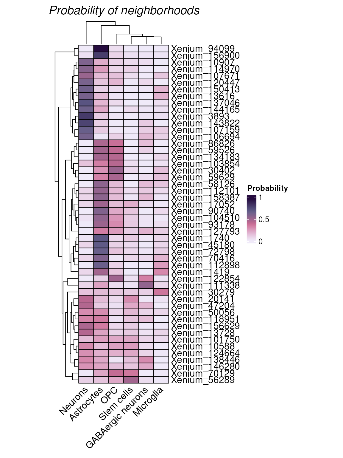
We can then merge the neighborhood results with the
SpatialExperiment object using mergeHoodSpe so
that we can conduct more neighborhood-related analysis.
tx_spe_sample_1 =  tx_spe_sample_1 |> mergeHoodSpe(hoods)

tx_spe_sample_1 <- calcMetrics(tx_spe_sample_1, pm_cols = colnames(hoods))

# Entropy and perplexity statistics are added to the object
tx_spe_sample_1
## # A SpatialExperiment-tibble abstraction: 31,938 × 27
## # Features = 541 | Cells = 31938 | Assays = counts, logcounts
## .cell sample_id cell_id transcript_id qv region in_tissue sizeFactor
## <chr> <fct> <fct> <dbl> <dbl> <fct> <lgl> <dbl>
## 1 Xenium_V1_… 1 125137 2.82e14 33.3 SSp-b… TRUE 0.779
## 2 Xenium_V1_… 1 5000 2.82e14 33.6 CA2 TRUE 0.929
## 3 Xenium_V1_… 1 67843 2.82e14 32.6 RSPd1 TRUE 0.333
## 4 Xenium_V1_… 1 134051 2.82e14 32.5 fiber… TRUE 0.572
## 5 Xenium_V1_… 1 93903 2.82e14 30.8 TEa2/3 TRUE 1.74
## 6 Xenium_V1_… 1 11074 2.82e14 32.0 MEZ TRUE 0.715
## 7 Xenium_V1_… 1 44945 2.82e14 32.5 alv TRUE 0.341
## 8 Xenium_V1_… 1 160596 2.82e14 30.8 SSs5 TRUE 0.862
## 9 Xenium_V1_… 1 125886 2.82e14 32.6 SSp-b… TRUE 0.228
## 10 Xenium_V1_… 1 30417 2.82e14 34.5 int TRUE 0.868
## # ℹ 31,928 more rows
## # ℹ 19 more variables: my_clusters <chr>, cell_type <chr>, Astrocytes <dbl>,
## # GABAergic.neurons <dbl>, Microglia <dbl>, Neurons <dbl>, OPC <dbl>,
## # Stem.cells <dbl>, entropy <dbl>, perplexity <dbl>, x <dbl>, y <dbl>,
## # PC1 <dbl>, PC2 <dbl>, PC3 <dbl>, PC4 <dbl>, PC5 <dbl>, UMAP1 <dbl>,
## # UMAP2 <dbl>Perplexity of 1 means the cell is located in a very distinct neighborhood, perplexity of 2 means the cell is located in a mixed neighborhood, and the probability is about 50% to 50%.
plotTissue(tx_spe_sample_1, size = 0.5, color = perplexity) +
scale_color_scico(palette = "tokyo")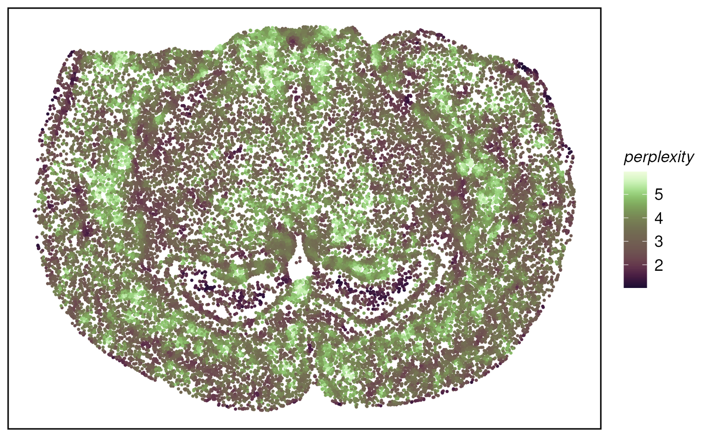 k-means algorithm based on neighbour composition
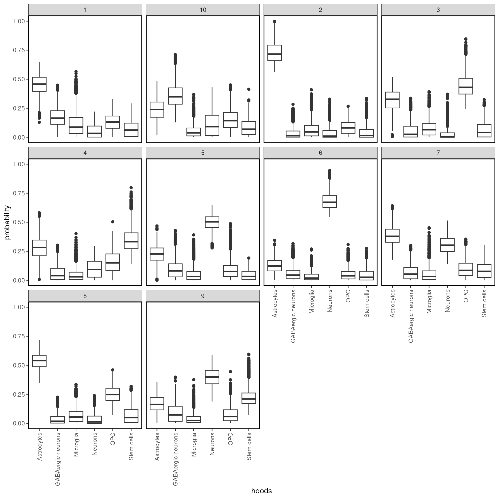
tx_spe_sample_1 <- clustByHood(tx_spe_sample_1, pm_cols = colnames(hoods), k = 10)## Warning: Quick-TRANSfer stage steps exceeded maximum (= 1596900)We can see what are the neighborhood distributions look like in each
cluster using plotProbDist.
tx_spe_sample_1 |>
  plotProbDist(
    pm_cols = colnames(hoods),
    by_cluster = TRUE,
    plot_all = TRUE,
    show_clusters = as.character(seq(99))
    )
The clusters can then be plot on the tissue using
plotissue
tx_spe_sample_1 |> plotTissue(color = clusters)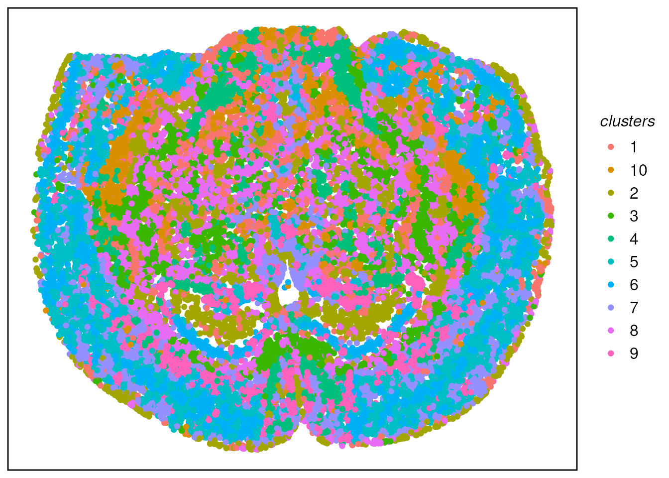
Session Information
## R version 4.6.0 (2026-04-24)
## Platform: x86_64-pc-linux-gnu
## Running under: Ubuntu 24.04.4 LTS
##
## Matrix products: default
## BLAS:   /usr/lib/x86_64-linux-gnu/openblas-pthread/libblas.so.3
## LAPACK: /usr/lib/x86_64-linux-gnu/openblas-pthread/libopenblasp-r0.3.26.so;  LAPACK version 3.12.0
##
## locale:
##  [1] LC_CTYPE=en_US.UTF-8       LC_NUMERIC=C
##  [3] LC_TIME=en_US.UTF-8        LC_COLLATE=en_US.UTF-8
##  [5] LC_MONETARY=en_US.UTF-8    LC_MESSAGES=en_US.UTF-8
##  [7] LC_PAPER=en_US.UTF-8       LC_NAME=C
##  [9] LC_ADDRESS=C               LC_TELEPHONE=C
## [11] LC_MEASUREMENT=en_US.UTF-8 LC_IDENTIFICATION=C
##
## time zone: UTC
## tzcode source: system (glibc)
##
## attached base packages:
## [1] stats4    stats     graphics  grDevices utils     datasets  methods
## [8] base
##
## other attached packages:
##  [1] scRNAseq_2.27.0                 MoleculeExperiment_1.13.0
##  [3] SingleR_2.15.0                  scico_1.5.0
##  [5] hoodscanR_1.11.0                tidySpatialExperiment_1.9.0
##  [7] SpatialExperiment_1.23.0        tidySummarizedExperiment_1.23.0
##  [9] tidySingleCellExperiment_1.23.0 ttservice_0.5.3
## [11] scran_1.41.0                    scater_1.41.1
## [13] scuttle_1.23.1                  SingleCellExperiment_1.35.1
## [15] SummarizedExperiment_1.43.0     Biobase_2.73.1
## [17] GenomicRanges_1.65.0            Seqinfo_1.3.0
## [19] IRanges_2.47.1                  S4Vectors_0.51.2
## [21] BiocGenerics_0.59.2             generics_0.1.4
## [23] MatrixGenerics_1.25.0           matrixStats_1.5.0
## [25] RColorBrewer_1.1-3              ggspavis_1.19.0
## [27] dittoSeq_1.25.0                 colorspace_2.1-2
## [29] tibble_3.3.1                    forcats_1.0.1
## [31] stringr_1.6.0                   glue_1.8.1
## [33] purrr_1.2.2                     tidyr_1.3.2
## [35] dplyr_1.2.1                     plotly_4.12.0
## [37] ggplot2_4.0.3
##
## loaded via a namespace (and not attached):
##   [1] fs_2.1.0                 ProtGenerics_1.45.0      bitops_1.0-9
##   [4] EBImage_4.55.0           doParallel_1.0.17        httr_1.4.8
##   [7] tools_4.6.0              alabaster.base_1.13.0    utf8_1.2.6
##  [10] R6_2.6.1                 HDF5Array_1.41.0         lazyeval_0.2.3
##  [13] uwot_0.2.4               mgcv_1.9-4               GetoptLong_1.1.1
##  [16] rhdf5filters_1.25.0      withr_3.0.2              gridExtra_2.3
##  [19] cli_3.6.6                textshaping_1.0.5        Cairo_1.7-0
##  [22] alabaster.se_1.13.0      labeling_0.4.3           sass_0.4.10
##  [25] S7_0.2.2                 ggridges_0.5.7           pkgdown_2.2.0
##  [28] Rsamtools_2.29.0         systemfonts_1.3.2        limma_3.69.1
##  [31] RSQLite_3.52.0           shape_1.4.6.1            BiocIO_1.23.3
##  [34] scrapper_1.7.3           Matrix_1.7-5             ggbeeswarm_0.7.3
##  [37] fansi_1.0.7              abind_1.4-8              terra_1.9-27
##  [40] lifecycle_1.0.5          yaml_2.3.12              edgeR_4.11.0
##  [43] tidygate_1.0.19          rhdf5_2.57.0             SparseArray_1.13.2
##  [46] BiocFileCache_3.3.0      grid_4.6.0               blob_1.3.0
##  [49] promises_1.5.0           dqrng_0.4.1              ExperimentHub_3.3.0
##  [52] crayon_1.5.3             lattice_0.22-9           beachmat_2.29.0
##  [55] cowplot_1.2.0            GenomicFeatures_1.65.0   cigarillo_1.3.0
##  [58] KEGGREST_1.53.0          magick_2.9.1             ComplexHeatmap_2.29.0
##  [61] pillar_1.11.1            knitr_1.51               metapod_1.21.0
##  [64] rjson_0.2.23             codetools_0.2-20         data.table_1.18.4
##  [67] vctrs_0.7.3              png_0.1-9                gypsum_1.9.0
##  [70] gtable_0.3.6             cachem_1.1.0             xfun_0.57
##  [73] S4Arrays_1.13.0          mime_0.13                ggside_0.4.1
##  [76] pheatmap_1.0.13          iterators_1.0.14         statmod_1.5.2
##  [79] bluster_1.23.0           ellipsis_0.3.3           nlme_3.1-169
##  [82] bit64_4.8.2              alabaster.ranges_1.13.0  filelock_1.0.3
##  [85] RcppAnnoy_0.0.23         GenomeInfoDb_1.49.0      bslib_0.11.0
##  [88] irlba_2.3.7              vipor_0.4.7              otel_0.2.0
##  [91] DBI_1.3.0                tidyselect_1.2.1         bit_4.6.0
##  [94] compiler_4.6.0           curl_7.1.0               httr2_1.2.2
##  [97] BiocNeighbors_2.7.2      h5mread_1.5.0            desc_1.4.3
## [100] DelayedArray_0.39.2      rtracklayer_1.73.0       scales_1.4.0
## [103] rappdirs_0.3.4           tiff_0.1-12              digest_0.6.39
## [106] fftwtools_0.9-11         alabaster.matrix_1.13.0  rmarkdown_2.31
## [109] XVector_0.53.0           htmltools_0.5.9          pkgconfig_2.0.3
## [112] jpeg_0.1-11              sparseMatrixStats_1.25.0 dbplyr_2.5.2
## [115] fastmap_1.2.0            ensembldb_2.37.0         GlobalOptions_0.1.4
## [118] rlang_1.2.0              htmlwidgets_1.6.4        UCSC.utils_1.9.0
## [121] shiny_1.13.0             farver_2.1.2             jquerylib_0.1.4
## [124] jsonlite_2.0.0           BiocParallel_1.47.0      BiocSingular_1.29.0
## [127] RCurl_1.98-1.18          magrittr_2.0.5           Rhdf5lib_2.1.0
## [130] Rcpp_1.1.1-1.1           viridis_0.6.5            stringi_1.8.7
## [133] alabaster.schemas_1.13.0 AnnotationHub_4.3.0      parallel_4.6.0
## [136] ggrepel_0.9.8            Biostrings_2.81.1        splines_4.6.0
## [139] circlize_0.4.18          locfit_1.5-9.12          igraph_2.3.1
## [142] ScaledMatrix_1.21.0      BiocVersion_3.24.0       XML_3.99-0.23
## [145] evaluate_1.0.5           BiocManager_1.30.27      foreach_1.5.2
## [148] httpuv_1.6.17            RANN_2.6.2               clue_0.3-68
## [151] alabaster.sce_1.13.0     BiocBaseUtils_1.15.1     rsvd_1.0.5
## [154] xtable_1.8-8             restfulr_0.0.16          AnnotationFilter_1.37.0
## [157] RSpectra_0.16-2          later_1.4.8              viridisLite_0.4.3
## [160] ragg_1.5.2               memoise_2.0.1            beeswarm_0.4.0
## [163] AnnotationDbi_1.75.0     GenomicAlignments_1.49.0 cluster_2.1.8.2
References
<mangiola.s at wehi.edu.au>↩︎