Solutions to exercises
Stefano Mangiola, South Australian immunoGENomics Cancer Institute1, Walter and Eliza Hall Institute2
Source:vignettes/Solutions.Rmd
Solutions.Rmd
library(spatialLIBD)
library(ExperimentHub)
library(scater)
library(ggplot2)
library(tidySpatialExperiment)
library(dplyr)

setClassUnion("ExpData", c("matrix", "SpatialExperiment"))

spatial_data <-
  ExperimentHub::ExperimentHub() |>
  spatialLIBD::fetch_data(eh = _, type = "spe")

names(libd_layer_colors) <- gsub("ayer", "", names(libd_layer_colors))

reducedDims(spatial_data) <- NULL
spatial_data <- spatial_data[, spatial_data$sample_id %in% c("151673", "151675", "151676")]
spatial_data <- spatial_data[, colData(spatial_data)$in_tissue == 1]

is_gene_mitochondrial <- grepl("(^MT-)|(^mt-)", rowData(spatial_data)$gene_name)
spatial_data <- scater::addPerCellQC(
  spatial_data,
  subsets = list(mito = is_gene_mitochondrial)
)
qc_mitochondrial_transcription <- colData(spatial_data)$subsets_mito_percent > 30
colData(spatial_data)$qc_mitochondrial_transcription <- qc_mitochondrial_transcription
Exercise 1.0
spot_counts <-
  colData(spatial_data) |>
  as.data.frame() |>
  group_by(sample_id) |>
  summarise(n_spots = n())

spot_counts
## # A tibble: 3 × 2
## sample_id n_spots
## <chr> <int>
## 1 151673 3639
## 2 151675 3592
## 3 151676 3460
spot_counts <-
  spot_counts |>
  mutate(pct_of_lowres = n_spots / 5000 * 100)

spot_counts
## # A tibble: 3 × 3
## sample_id n_spots pct_of_lowres
## <chr> <int> <dbl>
## 1 151673 3639 72.8
## 2 151675 3592 71.8
## 3 151676 3460 69.2Exercise 1.0.1
colData(spatial_data) |>
  ggplot(aes(subsets_mito_percent)) +
geom_density(aes(linetype = sample_id)) 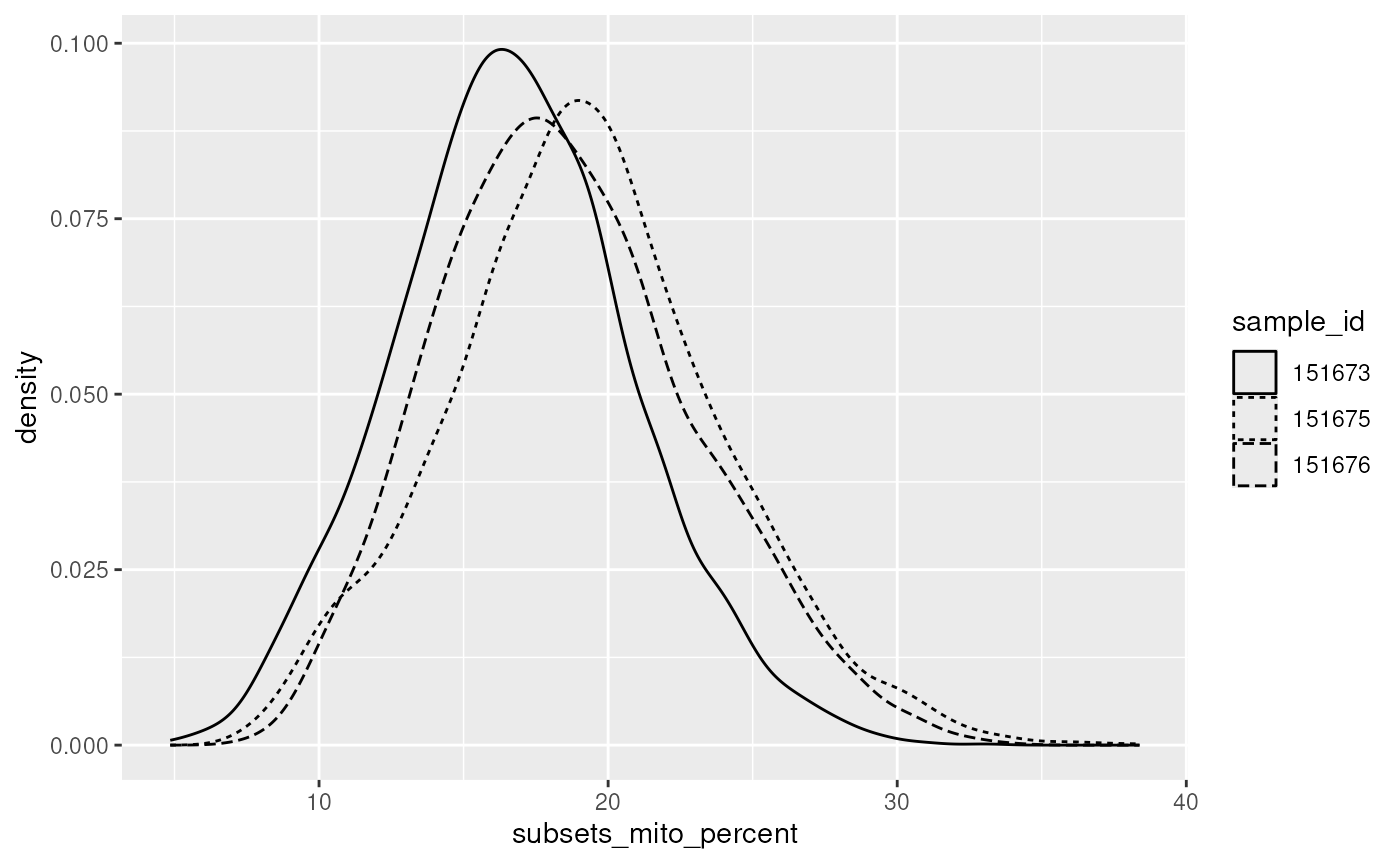
colData(spatial_data) |>
  ggplot(aes(subsets_mito_percent)) +
geom_density(aes(color = spatialLIBD, linetype = sample_id)) 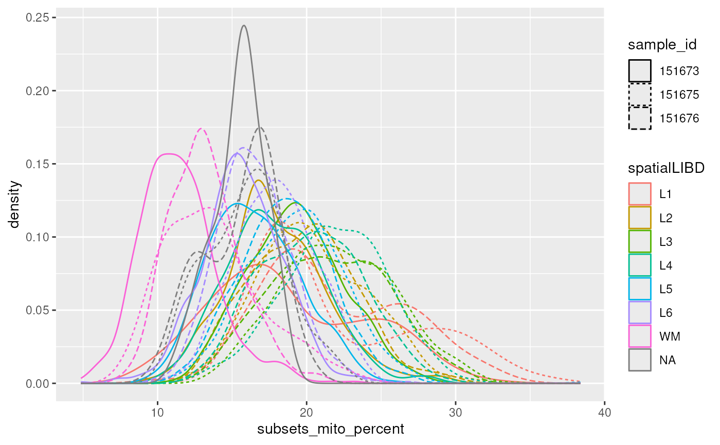
Exercise 1.0.2
##
## FALSE  TRUE
## 10652 39##
## FALSE TRUE
## 10599 92Exercise 1.1
# Label
colData(spatial_data)$macro_cluster = reducedDim(spatial_data, "UMAP")[,"UMAP1"] > -2.5

# Verify
scater::plotUMAP(spatial_data, colour_by = "macro_cluster", point_size = 0.2)

ggspavis::plotVisium(
  spatial_data,
  annotate = "macro_cluster",
  highlight = "in_tissue"
)
Exercise 1.2
spe_joint <- do.call(cbind, spatial_data_list)


 ggspavis::plotCoords(spe_joint, annotate = sprintf("%s", "clust_M0_lam0.2_k50_res0.7"), pal = pal) +
    facet_wrap(~sample_id) +
    theme(legend.position = "none") +
    labs(title = "BANKSY clusters")
spe_joint$has_changed =  !spe_joint$clust_M0_lam0.2_k50_res0.7 == spe_joint$clust_M0_lam0.2_k50_res0.7_smooth

plotSpotQC(
  spe_joint,
  plot_type = "spot",
  annotate = "has_changed",
) +
  facet_wrap(~sample_id)
Excercise 1.3
res_spatialLIBD = split(data.frame(res$mat), spatial_data_gene_name$sample_id, drop = TRUE )

lapply(res_spatialLIBD, function(x) plotCorrelationMatrix(as.matrix(x)))
Excercise 1.4
res_spatialLIBD = split(data.frame(res$mat), colData(spatial_data_gene_name)$spatialLIBD )

lapply(res_spatialLIBD, function(x) plotCorrelationMatrix(as.matrix(x[,-10])))
Excercise 1.5
# 1. Microglia + Neurons
is_microglia_neuron <- mat_df$Microglia > 0.1 &
                       mat_df$Neurons   > 0.1 &
                       (mat_df$Microglia + mat_df$Neurons) > 0.4
spatial_data$is_microglia_neuron <- is_microglia_neuron

ggspavis::plotCoords(spatial_data, annotate = "is_microglia_neuron") +
  facet_wrap(~sample_id) +
  scale_color_manual(values = c("TRUE" = "red", "FALSE" = "grey")) +
  theme(legend.position = "none") +
  labs(title = "Microglia + Neurons")


# 2. Astrocytes + Stem cells
# note the space in the column name — use backticks
is_astrocyte_stem <- mat_df$Astrocytes     > 0.1 &
                     mat_df$`Stem cells`   > 0.1 &
                     (mat_df$Astrocytes + mat_df$`Stem cells`) > 0.4
spatial_data$is_astrocyte_stem <- is_astrocyte_stem

ggspavis::plotCoords(spatial_data, annotate = "is_astrocyte_stem") +
  facet_wrap(~sample_id) +
  scale_color_manual(values = c("TRUE" = "blue", "FALSE" = "grey")) +
  theme(legend.position = "none") +
  labs(title = "Astrocytes + Stem cells")
Excercise 1.6 :::
# Get reference
library(cellNexus)
library(HDF5Array)

tmp_file_path = tempfile()

DelayedArray::setAutoBlockSize(size=1e9)

brain_reference =

  # Query metadata across 30M cells
  get_metadata() |>

  # Filter your data of interest
  dplyr::filter(tissue=="dorsolateral prefrontal cortex", disease == "normal") |>

  # Collect pseudobulk as SummarizedExperiment
  get_pseudobulk() |>

  # Normalise for Spotlight
  scuttle::logNormCounts() |>

  # Save for fast reading
  HDF5Array::saveHDF5SummarizedExperiment(tmp_file_path, replace = TRUE, verbose = TRUE)
library(HDF5Array)

brain_reference = HDF5Array::loadHDF5SummarizedExperiment(tmp_file_path)

my_metadata = colData(brain_reference)

knitr::kable(head(my_metadata), format = "html")
These are the cell types included in our reference, and the number of pseudobulk samples we have for each cell type.
table(brain_reference$cell_types)These are the number of samples we have for each of the three data sets.
table(brain_reference$dataset_id)The collection_id can be used to gather information on
the cell database. e.g. https://cellxgene.cziscience.com/collections/
table(brain_reference$collection_id)Exercise 2.1
# Get top variable genes
genes <- !grepl(pattern = "^Rp[l|s]|Mt", x = rownames(spatial_data))
hvg =
  spatial_data |>
  scran::modelGeneVar(subset.row = genes, block = spatial_data$sample_id) |>
  scran::getTopHVGs(n = 1000)

# Calculate PCA
spatial_data |>

  scuttle::logNormCounts() |>
  scater::runPCA(subset_row = hvg) |>

  # Calculate UMAP
  scater::runUMAP(dimred = "PCA") |>

  # Filter one sample
  filter(in_tissue, sample_id=="151673") |>

  # Gate based on tissue morphology
  tidySpatialExperiment::gate(alpha = 0.1,colour = "spatialLIBD") |>

  # Plot
  scater::plotUMAP(colour_by = ".gated")
Exercise 2.2
rowData(spatial_data) |>
  as_tibble() |>
  filter( gene_name == "PECAM1")

gene = "ENSG00000261371"

spatial_data |>

  # Join the feature
  join_features(gene, shape="wide", assay = "logcounts") |>

  # Calculate the quantile
  mutate(my_quantile = quantile(ENSG00000261371, 0.99)) |>
  # mutate(my_quantile = ENSG00000261371 > 0) |> # A possibility

  # Label the pixels
  mutate(PECAM1_positive = ENSG00000261371 >= my_quantile) |>

  # Plot
  ggspavis::plotCoords(annotate = "PECAM1_positive") +
  facet_wrap(~sample_id)
Exercise 2.2.1
spatial_data |>
  mutate(qc_mitochondrial_transcription = scater::isOutlier(subsets_mito_percent, type="higher")) |>
  count(qc_mitochondrial_transcription)
## tidySingleCellExperiment says: A data frame is returned for independent data analysis.## Warning: `when()` was deprecated in purrr 1.0.0.
## ℹ Please use `if` instead.
## ℹ The deprecated feature was likely used in the tidySpatialExperiment package.
## Please report the issue at
## <https://github.com/william-hutchison/tidySpatialExperiment/issues>.
## This warning is displayed once per session.
## Call `lifecycle::last_lifecycle_warnings()` to see where this warning was
## generated.## # A tibble: 2 × 2
## qc_mitochondrial_transcription n
## <otlr.flt> <int>
## 1 FALSE 10652
## 2 TRUE 39
spatial_data |>
  count(qc_mitochondrial_transcription)
## tidySingleCellExperiment says: A data frame is returned for independent data analysis.## # A tibble: 2 × 2
## qc_mitochondrial_transcription n
## <lgl> <int>
## 1 FALSE 10599
## 2 TRUE 92Excercise 2.3
library(tidySummarizedExperiment)
library(tidybulk)

differential_analysis =
  spatial_data |>
  mutate(
    dead =

      # Stringent threshold
      subsets_mito_percent > 20 |
      sum < 700 |
      detected < 500
  ) |>
  aggregate_cells(c(sample_id, spatialLIBD, dead)) |>
  keep_abundant(factor_of_interest = c(dead)) |>
  nest(data = - spatialLIBD) |>

  # filter regions having both alive and dead cells
  filter(  map_int(data, ~ .x |> distinct(sample_id, dead) |> nrow() ) == 6 ) |>

  # DE analyses
  mutate(data = map(
    data,
    test_differential_abundance,
    ~ dead + sample_id,
    method = "edgeR_quasi_likelihood",
    test_above_log2_fold_change = log(2)
  ))

differential_analysis |>
  mutate(data = map(data, pivot_transcript)) |>
  unnest(data) |>
  filter(FDR<0.05)
Excercise 2.4
rownames(spatial_data_filtered) = rowData(spatial_data_filtered)$gene_name

marker_genes_of_amyloid_plaques = c("APP", "PSEN1", "PSEN2", "CLU", "APOE", "CD68", "ITGAM", "AIF1")

spatial_data_filtered |>

# Join the features
  join_features(marker_genes_of_amyloid_plaques, shape = "wide") |>

  # Rescaling
  mutate(across(any_of(marker_genes_of_amyloid_plaques), scales::rescale)) |>

# Summarising signature
  mutate(amyloid_plaques_signature  = APP + PSEN1 + PSEN2 + CLU + APOE + CD68 + ITGAM + AIF1) |>

# Plotting
  ggspavis::plotCoords(
    annotate = "amyloid_plaques_signature"
  ) +
  facet_wrap(~sample_id)
Exercise 3.1
# Base R
out_in_table <- table(is.na(tx_small_region$cell))
ratio_out_in <- out_in_table[2] / c(out_in_table[1] + out_in_table[2])
ratio_out_in

# Tidyverse
tx_small_region |>
  summarise(
    ratio_out_in = sum(is.na(cell)) / n()
  )

tx_small_region |>
  summarise(
    cytoplasm = count(overlaps_nucleus == "0" & !is.na(cell)),
    nucleus = count(overlaps_nucleus == "1" & !is.na(cell)),
    cytoplasm_ptc = cytoplasm / (cytoplasm + nucleus) * 100
  )
Exercise 3.2
mgs <- scran::scoreMarkers(
  tx_spe_sample_1,
  groups = tx_spe_sample_1$clusters,

  # Omit mitochondrial genes and keep all the genes in spatial
  subset.row =
    grep("NegControl.+|BLANK.+", top.hvgs, value=TRUE, invert=TRUE)
)

# Select the most informative markers
mgs_df <- lapply(names(mgs), function(i) {
  x <- mgs[[i]]

  # Filter and keep relevant marker genes, those with AUC > 0.8
  x <- x[x$mean.AUC > 0.8, ]

  # Sort the genes from highest to lowest weight
  x <- x[order(x$mean.AUC, decreasing = TRUE), ]

  # Add gene and cluster id to the dataframe
  x$gene <- rownames(x)
  x$cluster <- i
  data.frame(x)
})

head(mgs_df[[1]])

tx_spe_sample_1 |>
  plotReducedDim("UMAP", colour_by="Gjc3")
Exercise 3.3
library(Banksy)

# scale the counts, without log transformation
tx_spe_sample_1 = tx_spe_sample_1 |> logNormCounts(log=FALSE, name = "normcounts")
Highly-variable genes
The Banksy documentation, suggest the use of Seurat for
the detection of highly variable genes.
library(Seurat)

"NegControl.+|BLANK.+"

tx_spe_sample_1_seu =
  as.Seurat(tx_spe_sample_1, data = NULL)

genes <- !grepl(pattern = "NegControl.+|BLANK.+", x = rownames(tx_spe_sample_1_seu))


tx_spe_sample_1_seu = tx_spe_sample_1_seu[genes,]

tx_spe_sample_1_seu = tx_spe_sample_1_seu |>
  NormalizeData(scale.factor = 5000, normalization.method = 'RC')


# Compute HVGs
hvgs <-  VariableFeatures(FindVariableFeatures(tx_spe_sample_1_seu, nfeatures = 2000))


rm(tx_spe_sample_1_seu)

head(hvgs)
We now split the data by sample, to compute the neighbourhood matrices.
# Convert to list
tx_spe_sample_1_banksy = tx_spe_sample_1[hvgs,]

# Compute the component neighborhood matrices
tx_spe_sample_1_banksy = tx_spe_sample_1_banksy |>
  computeBanksy(
  assay_name = "normcounts"
  )
Here, we perform PCA using the BANKSY algorithm on the joint dataset. The group argument specifies how to treat different samples, ensuring that features are scaled separately per sample group to account for variations among them.
tx_spe_sample_1_banksy <- runBanksyPCA( # Run PCA on the Banskly matrix
  tx_spe_sample_1_banksy,
  lambda = 0.2, # spatial weighting parameter. Larger values (e.g. 0.8) incorporate more spatial neighborhood
  seed = 42
)
Once the dimensional reduction is complete, we cluster the spots
across all samples and use connectClusters to visually
compare these new BANKSY clusters against manual annotations.
tx_spe_sample_1_banksy <- clusterBanksy( # clustering on the principal components computed on the BANKSY matrix
  tx_spe_sample_1_banksy,
  lambda = 0.2, # spatial weighting parameter. Larger values (e.g. 0.8) incorporate more spatial neighborhood
  resolution = 0.7, # numeric vector specifying resolution used for clustering (louvain / leiden).
  seed = 42
)
As an optional step, we smooth the cluster labels for each sample independently, which can enhance the visual coherence of clusters, especially in heterogeneous biological samples.
From SpiceMix paper Chidester et al., 2023
tx_spe_sample_1_banksy_smoothed = tx_spe_sample_1_banksy |>
 smoothLabels(
  cluster_names = "clust_M0_lam0.2_k50_res0.7",
  k = 6L,
  verbose = FALSE
)
The raw and smoothed cluster labels are stored in the
colData slot of each SingleCellExperiment or
SpatialExperiment object.
Visualising Clusters and Annotations on Spatial Coordinates: We utilise the ggspavis package to visually map BANKSY clusters and manual annotations onto the spatial coordinates of the dataset, providing a comprehensive visual overview of spatial and clustering data relationships.
# Use scater:::.get_palette('tableau10medium')

 ggspavis::plotCoords(
   tx_spe_sample_1_banksy,
   annotate = "clust_M0_lam0.2_k50_res0.7"
  ) +
    guides(color = "none") +
    labs(title = "BANKSY clusters")

 ggspavis::plotCoords(
   tx_spe_sample_1_banksy_smoothed,
   annotate = "clust_M0_lam0.2_k50_res0.7_smooth"
  ) +
    guides(color = "none") +
    labs(title = "BANKSY clusters smoothed")

# ggspavis::plotCoords(
#   tx_spe_sample_1_banksy,
#   annotate = "clusters"
#   ) +
#     guides(color = "none") +
#     labs(title = "cell clustering")

ggspavis::plotCoords(
tx_spe_sample_1_banksy,
annotate = "region"
) +
      scale_color_manual(values = colorRampPalette( brewer.pal(9,"Set1") )(150) ) +
    guides(color = "none") +
labs(title = "ground truth")<mangiola.s at wehi.edu.au>↩︎