Tidy spatial analyses

Session 2: Tidying spatial data

Introduction to tidyomics

tidyomics represents a significant advancement in bioinformatics analysis by bridging the gap between Bioconductor and the tidyverse ecosystem. This integration provides several key benefits:

Unified Analysis Framework: Combines the power of Bioconductor’s specialized biological data structures with tidyverse’s intuitive data manipulation
Maintained Compatibility: Preserves original data containers and methods, ensuring long-term support
Enhanced Workflow Efficiency: Enables streamlined analysis pipelines using familiar tidyverse syntax

The ecosystem includes several specialized packages: - tidySummarizedExperiment: For bulk RNA-seq analysis - tidySingleCellExperiment: For single-cell data - tidySpatialExperiment: For spatial transcriptomics - Additional tools: plyranges, nullranges, tidyseurat, tidybulk, tidytof

tidySpatialWorkshop tidy transcriptomic manifesto

tidyomics is an interoperable software ecosystem that bridges Bioconductor and the tidyverse. tidyomics is installable with a single homonymous meta-package. This ecosystem includes three new packages: tidySummarizedExperiment, tidySingleCellExperiment, and tidySpatialExperiment, and five publicly available R packages: plyranges, nullranges, tidyseurat, tidybulk, tidytof. Importantly, tidyomics leaves the original data containers and methods unaltered, ensuring compatibility with existing software, maintainability and long-term Bioconductor support.

tidyomics is presented in “The tidyomics ecosystem: Enhancing omic data analyses” Hutchison and Keyes et al., 2025

Slides

Installation

let’s make sure we get the latest packages available on github

# In May 2025, the following packages should be installed from github repositories, to use the latest features. In case you have them pre installed, run the following command
BiocManager::install(c("lmweber/ggspavis", 
                       "stemangiola/tidySummarizedExperiment", 
                        "stemangiola/tidySingleCellExperiment", 
                       "william-hutchison/tidySpatialExperiment", 
                       "stemangiola/tidybulk", 
                       "stemangiola/tidygate"), 
                     update = FALSE)

Important: Please restart your R session after installation to ensure the updated packages are loaded correctly.

Let’s load the libraries needed for this session

library(SpatialExperiment)

# Tidyverse library(tidyverse)
library(ggplot2)
library(plotly)
library(dplyr)
library(tidyr)
library(purrr)
library(glue) # sprintf
library(stringr)

# Plotting
library(colorspace)
library(dittoSeq)
library(ggspavis)

# Analysis
library(scuttle)
library(scater)
library(scran)

Similarly to Section 2, this section uses spatialLIBD and ExperimentHub packages to gather spatial transcriptomics data.

doi: 10.1038/s41593-020-00787-0

# From https://bioconductor.org/packages/devel/bioc/vignettes/Banksy/inst/doc/multi-sample.html
library(spatialLIBD)
library(ExperimentHub)

spatial_data <- 
  ExperimentHub::ExperimentHub() |> 
  spatialLIBD::fetch_data( eh = _, type = "spe")

# Clear the reductions
reducedDims(spatial_data) = NULL 

# Make cell ID unique
colnames(spatial_data)  = paste0(colnames(spatial_data), colData(spatial_data)$sample_id)
rownames(spatialCoords(spatial_data)) = colnames(spatial_data) # Bug?

# Display the object
spatial_data

## class: SpatialExperiment 
## dim: 33538 47681 
## metadata(0):
## assays(2): counts logcounts
## rownames(33538): ENSG00000243485 ENSG00000237613 ... ENSG00000277475
##   ENSG00000268674
## rowData names(9): source type ... gene_search is_top_hvg
## colnames(47681): AAACAACGAATAGTTC-1151507 AAACAAGTATCTCCCA-1151507 ...
##   TTGTTTCCATACAACT-1151676 TTGTTTGTGTAAATTC-1151676
## colData names(69): sample_id Cluster ... array_row array_col
## reducedDimNames(0):
## mainExpName: NULL
## altExpNames(0):
## spatialCoords names(2) : pxl_col_in_fullres pxl_row_in_fullres
## imgData names(4): sample_id image_id data scaleFactor

If ExperimentHub should not work. The spatial_data object from the previous code block can be downloaded from Zenodo - 10.5281/zenodo.11233385

Working with tidySpatialExperiment

The tidySpatialExperiment package creates a bridge between SpatialExperiment objects and the tidyverse ecosystem. It provides:

A tidy data view of SpatialExperiment objects
Compatible dplyr, tidyr, ggplot and plotly functions
Seamless integration with existing SpatialExperiment functionality

1. tidySpatialExperiment package

tidySpatialExperiment provides a bridge between the SpatialExperiment single-cell package and the tidyverse [@wickham2019welcome]. It creates an invisible layer that enables viewing the SpatialExperiment object as a tidyverse tibble, and provides SpatialExperiment-compatible dplyr, tidyr, ggplot and plotly functions.

If we load the tidySpatialExperiment package and then view the single cell data, it now displays as a tibble.

library(tidySpatialExperiment)

spatial_data

## # A SpatialExperiment-tibble abstraction: 47,681 × 72
## # Features = 33538 | Cells = 47681 | Assays = counts, logcounts
##    .cell           sample_id Cluster sum_umi sum_gene subject position replicate
##    <chr>           <chr>       <int>   <dbl>    <int> <chr>   <chr>    <chr>    
##  1 AAACAACGAATAGT… 151507          6     948      727 Br5292  0        1        
##  2 AAACAAGTATCTCC… 151507          3    4261     2170 Br5292  0        1        
##  3 AAACAATCTACTAG… 151507          2    1969     1093 Br5292  0        1        
##  4 AAACACCAATAACT… 151507          5    3368     1896 Br5292  0        1        
##  5 AAACAGCTTTCAGA… 151507          1    2981     1620 Br5292  0        1        
##  6 AAACAGGGTCTATA… 151507          2    4114     2135 Br5292  0        1        
##  7 AAACAGTGTTCCTG… 151507          6    2077     1350 Br5292  0        1        
##  8 AAACATTTCCCGGA… 151507          5    4535     2347 Br5292  0        1        
##  9 AAACCACTACACAG… 151507          4    6577     2911 Br5292  0        1        
## 10 AAACCCGAACGAAA… 151507          3    5029     2393 Br5292  0        1        
## # ℹ 47,671 more rows
## # ℹ 64 more variables: subject_position <chr>, discard <lgl>, key <chr>,
## #   cell_count <int>, SNN_k50_k4 <int>, SNN_k50_k5 <int>, SNN_k50_k6 <int>,
## #   SNN_k50_k7 <int>, SNN_k50_k8 <int>, SNN_k50_k9 <int>, SNN_k50_k10 <int>,
## #   SNN_k50_k11 <int>, SNN_k50_k12 <int>, SNN_k50_k13 <int>, SNN_k50_k14 <int>,
## #   SNN_k50_k15 <int>, SNN_k50_k16 <int>, SNN_k50_k17 <int>, SNN_k50_k18 <int>,
## #   SNN_k50_k19 <int>, SNN_k50_k20 <int>, SNN_k50_k21 <int>, …

Data interface, display

If we want to revert to the standard SpatialExperiment view we can do that.

options("restore_SpatialExperiment_show" = TRUE)
spatial_data

## class: SpatialExperiment 
## dim: 33538 47681 
## metadata(0):
## assays(2): counts logcounts
## rownames(33538): ENSG00000243485 ENSG00000237613 ... ENSG00000277475
##   ENSG00000268674
## rowData names(9): source type ... gene_search is_top_hvg
## colnames(47681): AAACAACGAATAGTTC-1151507 AAACAAGTATCTCCCA-1151507 ...
##   TTGTTTCCATACAACT-1151676 TTGTTTGTGTAAATTC-1151676
## colData names(69): sample_id Cluster ... array_row array_col

If we want to revert back to tidy SpatialExperiment view we can.

options("restore_SpatialExperiment_show" = FALSE)
spatial_data

## # A SpatialExperiment-tibble abstraction: 47,681 × 72
## # Features = 33538 | Cells = 47681 | Assays = counts, logcounts
##    .cell           sample_id Cluster sum_umi sum_gene subject position replicate
##    <chr>           <chr>       <int>   <dbl>    <int> <chr>   <chr>    <chr>    
##  1 AAACAACGAATAGT… 151507          6     948      727 Br5292  0        1        
##  2 AAACAAGTATCTCC… 151507          3    4261     2170 Br5292  0        1        
##  3 AAACAATCTACTAG… 151507          2    1969     1093 Br5292  0        1        
##  4 AAACACCAATAACT… 151507          5    3368     1896 Br5292  0        1        
##  5 AAACAGCTTTCAGA… 151507          1    2981     1620 Br5292  0        1        
##  6 AAACAGGGTCTATA… 151507          2    4114     2135 Br5292  0        1        
##  7 AAACAGTGTTCCTG… 151507          6    2077     1350 Br5292  0        1        
##  8 AAACATTTCCCGGA… 151507          5    4535     2347 Br5292  0        1        
##  9 AAACCACTACACAG… 151507          4    6577     2911 Br5292  0        1        
## 10 AAACCCGAACGAAA… 151507          3    5029     2393 Br5292  0        1        
## # ℹ 47,671 more rows
## # ℹ 64 more variables: subject_position <chr>, discard <lgl>, key <chr>,
## #   cell_count <int>, SNN_k50_k4 <int>, SNN_k50_k5 <int>, SNN_k50_k6 <int>,
## #   SNN_k50_k7 <int>, SNN_k50_k8 <int>, SNN_k50_k9 <int>, SNN_k50_k10 <int>,
## #   SNN_k50_k11 <int>, SNN_k50_k12 <int>, SNN_k50_k13 <int>, SNN_k50_k14 <int>,
## #   SNN_k50_k15 <int>, SNN_k50_k16 <int>, SNN_k50_k17 <int>, SNN_k50_k18 <int>,
## #   SNN_k50_k19 <int>, SNN_k50_k20 <int>, SNN_k50_k21 <int>, …

Note that rows in this context refers to rows of the abstraction, not rows of the SpatialExperiment which correspond to genes tidySpatialExperiment prioritizes cells as the units of observation in the abstraction, while the full dataset, including measurements of expression of all genes, is still available “in the background”.

Original behaviour is preserved

The tidy representation behaves exactly as a native SpatialExperiment. It can be interacted with using SpatialExperiment commands such as assays.

assays(spatial_data)

## List of length 2
## names(2): counts logcounts

2. Tidyverse commands

We can also interact with our object as we do with any tidyverse tibble. We can use tidyverse commands, such as filter, select and mutate to explore the tidySpatialExperiment object. Some examples are shown below and more can be seen at the tidySpatialExperiment website.

Select

We can use select to view columns, for example, to see the filename, total cellular RNA abundance and cell phase.

If we use select we will also get any view-only columns returned, such as the UMAP columns generated during the preprocessing.

spatial_data |> select(.cell, sample_id, in_tissue, spatialLIBD)

## # A SpatialExperiment-tibble abstraction: 47,681 × 6
## # Features = 33538 | Cells = 47681 | Assays = counts, logcounts
##    .cell   sample_id in_tissue spatialLIBD pxl_col_in_fullres pxl_row_in_fullres
##    <chr>   <chr>     <lgl>     <fct>                    <dbl>              <dbl>
##  1 AAACAA… 151507    TRUE      L1                        3276               2514
##  2 AAACAA… 151507    TRUE      L3                        9178               8520
##  3 AAACAA… 151507    TRUE      L1                        5133               2878
##  4 AAACAC… 151507    TRUE      WM                        3462               9581
##  5 AAACAG… 151507    TRUE      L6                        2779               7663
##  6 AAACAG… 151507    TRUE      L6                        3053               8143
##  7 AAACAG… 151507    TRUE      WM                        5109              11263
##  8 AAACAT… 151507    TRUE      L5                        8830               9837
##  9 AAACCA… 151507    TRUE      L3                       10228               2894
## 10 AAACCC… 151507    TRUE      L3                       10075               7924
## # ℹ 47,671 more rows

Note that some columns are always displayed no matter whet. These column include special slots in the objects such as reduced dimensions, spatial coordinates (mandatory for SpatialExperiment), and sample identifier (mandatory for SpatialExperiment).

Although the select operation can be used as a display tool, to explore our object, it updates the SpatialExperiment metadata, subsetting the desired columns.

spatial_data |> 
  select(.cell, sample_id, in_tissue, spatialLIBD) |> 
  colData()

## DataFrame with 47681 rows and 3 columns
##                            sample_id in_tissue spatialLIBD
##                          <character> <logical>    <factor>
## AAACAACGAATAGTTC-1151507      151507      TRUE          L1
## AAACAAGTATCTCCCA-1151507      151507      TRUE          L3
## AAACAATCTACTAGCA-1151507      151507      TRUE          L1
## AAACACCAATAACTGC-1151507      151507      TRUE          WM
## AAACAGCTTTCAGAAG-1151507      151507      TRUE          L6
## ...                              ...       ...         ...
## TTGTTGTGTGTCAAGA-1151676      151676      TRUE          L6
## TTGTTTCACATCCAGG-1151676      151676      TRUE          WM
## TTGTTTCATTAGTCTA-1151676      151676      TRUE          WM
## TTGTTTCCATACAACT-1151676      151676      TRUE          L6
## TTGTTTGTGTAAATTC-1151676      151676      TRUE          L1

To select columns of interest, we can use tidyverse powerful pattern-matching tools. For example, using the method contains to select

spatial_data |> 
  select(.cell, contains("sum"))

## # A SpatialExperiment-tibble abstraction: 47,681 × 6
## # Features = 33538 | Cells = 47681 | Assays = counts, logcounts
##    .cell        sum_umi sum_gene sample_id pxl_col_in_fullres pxl_row_in_fullres
##    <chr>          <dbl>    <int> <chr>                  <dbl>              <dbl>
##  1 AAACAACGAAT…     948      727 151507                  3276               2514
##  2 AAACAAGTATC…    4261     2170 151507                  9178               8520
##  3 AAACAATCTAC…    1969     1093 151507                  5133               2878
##  4 AAACACCAATA…    3368     1896 151507                  3462               9581
##  5 AAACAGCTTTC…    2981     1620 151507                  2779               7663
##  6 AAACAGGGTCT…    4114     2135 151507                  3053               8143
##  7 AAACAGTGTTC…    2077     1350 151507                  5109              11263
##  8 AAACATTTCCC…    4535     2347 151507                  8830               9837
##  9 AAACCACTACA…    6577     2911 151507                 10228               2894
## 10 AAACCCGAACG…    5029     2393 151507                 10075               7924
## # ℹ 47,671 more rows

Filter

We can use filter to subset rows, for example, to keep our three samples we are going to work with.

We just display the dimensions of the dataset before filtering

ncol(spatial_data)

## [1] 47681

spatial_data = 
  spatial_data |> 
  filter(sample_id %in% c("151673", "151675", "151676"))

spatial_data

## # A SpatialExperiment-tibble abstraction: 10,691 × 72
## # Features = 33538 | Cells = 10691 | Assays = counts, logcounts
##    .cell           sample_id Cluster sum_umi sum_gene subject position replicate
##    <chr>           <chr>       <int>   <dbl>    <int> <chr>   <chr>    <chr>    
##  1 AAACAAGTATCTCC… 151673          7    8458     3586 Br8100  0        1        
##  2 AAACAATCTACTAG… 151673          4    1667     1150 Br8100  0        1        
##  3 AAACACCAATAACT… 151673          8    3769     1960 Br8100  0        1        
##  4 AAACAGAGCGACTC… 151673          6    5433     2424 Br8100  0        1        
##  5 AAACAGCTTTCAGA… 151673          3    4278     2264 Br8100  0        1        
##  6 AAACAGGGTCTATA… 151673          3    4004     2178 Br8100  0        1        
##  7 AAACAGTGTTCCTG… 151673          8    2376     1432 Br8100  0        1        
##  8 AAACATTTCCCGGA… 151673          5    8171     3456 Br8100  0        1        
##  9 AAACCCGAACGAAA… 151673          7   12723     4638 Br8100  0        1        
## 10 AAACCGGGTAGGTA… 151673          1    1294      888 Br8100  0        1        
## # ℹ 10,681 more rows
## # ℹ 64 more variables: subject_position <chr>, discard <lgl>, key <chr>,
## #   cell_count <int>, SNN_k50_k4 <int>, SNN_k50_k5 <int>, SNN_k50_k6 <int>,
## #   SNN_k50_k7 <int>, SNN_k50_k8 <int>, SNN_k50_k9 <int>, SNN_k50_k10 <int>,
## #   SNN_k50_k11 <int>, SNN_k50_k12 <int>, SNN_k50_k13 <int>, SNN_k50_k14 <int>,
## #   SNN_k50_k15 <int>, SNN_k50_k16 <int>, SNN_k50_k17 <int>, SNN_k50_k18 <int>,
## #   SNN_k50_k19 <int>, SNN_k50_k20 <int>, SNN_k50_k21 <int>, …

Here we confirm that the tidy R manipulation has changed the underlining object.

ncol(spatial_data)

## [1] 10691

In comparison the base-R method recalls the variable multiple times

spatial_data = spatial_data[,spatial_data$sample_id %in% c("151673", "151675", "151676")]

Or for example, to see just the rows for the cells in spatialLIBD region L1.

spatial_data |> dplyr::filter(sample_id == "151673", spatialLIBD == "L1")

## # A SpatialExperiment-tibble abstraction: 273 × 72
## # Features = 33538 | Cells = 273 | Assays = counts, logcounts
##    .cell           sample_id Cluster sum_umi sum_gene subject position replicate
##    <chr>           <chr>       <int>   <dbl>    <int> <chr>   <chr>    <chr>    
##  1 AAACAATCTACTAG… 151673          4    1667     1150 Br8100  0        1        
##  2 AAAGGTAAGCTGTA… 151673          1    3996     1932 Br8100  0        1        
##  3 AAATGTGGGTGCTC… 151673          1    2242     1172 Br8100  0        1        
##  4 AAATTGCGGCGGTT… 151673          1    1896     1213 Br8100  0        1        
##  5 AACACGCGGCCGCG… 151673          1    1825     1127 Br8100  0        1        
##  6 AACATTGGTCAGCC… 151673          1    1808     1148 Br8100  0        1        
##  7 AACGTAGTCTACCC… 151673          4    2870     1693 Br8100  0        1        
##  8 AACTAGCGTATCGC… 151673          1    1585      923 Br8100  0        1        
##  9 AACTCGATAAACAC… 151673          1    2138     1316 Br8100  0        1        
## 10 AACTCGATGGCGCA… 151673          1    1404      858 Br8100  0        1        
## # ℹ 263 more rows
## # ℹ 64 more variables: subject_position <chr>, discard <lgl>, key <chr>,
## #   cell_count <int>, SNN_k50_k4 <int>, SNN_k50_k5 <int>, SNN_k50_k6 <int>,
## #   SNN_k50_k7 <int>, SNN_k50_k8 <int>, SNN_k50_k9 <int>, SNN_k50_k10 <int>,
## #   SNN_k50_k11 <int>, SNN_k50_k12 <int>, SNN_k50_k13 <int>, SNN_k50_k14 <int>,
## #   SNN_k50_k15 <int>, SNN_k50_k16 <int>, SNN_k50_k17 <int>, SNN_k50_k18 <int>,
## #   SNN_k50_k19 <int>, SNN_k50_k20 <int>, SNN_k50_k21 <int>, …

Flexible, more powerful filters with stringr

spatial_data |> 
  dplyr::filter(
    subject |> str_detect("Br[0-9]1"), 
    spatialLIBD == "L1"
  )

## # A SpatialExperiment-tibble abstraction: 890 × 72
## # Features = 33538 | Cells = 890 | Assays = counts, logcounts
##    .cell           sample_id Cluster sum_umi sum_gene subject position replicate
##    <chr>           <chr>       <int>   <dbl>    <int> <chr>   <chr>    <chr>    
##  1 AAACAATCTACTAG… 151673          4    1667     1150 Br8100  0        1        
##  2 AAAGGTAAGCTGTA… 151673          1    3996     1932 Br8100  0        1        
##  3 AAATGTGGGTGCTC… 151673          1    2242     1172 Br8100  0        1        
##  4 AAATTGCGGCGGTT… 151673          1    1896     1213 Br8100  0        1        
##  5 AACACGCGGCCGCG… 151673          1    1825     1127 Br8100  0        1        
##  6 AACATTGGTCAGCC… 151673          1    1808     1148 Br8100  0        1        
##  7 AACGTAGTCTACCC… 151673          4    2870     1693 Br8100  0        1        
##  8 AACTAGCGTATCGC… 151673          1    1585      923 Br8100  0        1        
##  9 AACTCGATAAACAC… 151673          1    2138     1316 Br8100  0        1        
## 10 AACTCGATGGCGCA… 151673          1    1404      858 Br8100  0        1        
## # ℹ 880 more rows
## # ℹ 64 more variables: subject_position <chr>, discard <lgl>, key <chr>,
## #   cell_count <int>, SNN_k50_k4 <int>, SNN_k50_k5 <int>, SNN_k50_k6 <int>,
## #   SNN_k50_k7 <int>, SNN_k50_k8 <int>, SNN_k50_k9 <int>, SNN_k50_k10 <int>,
## #   SNN_k50_k11 <int>, SNN_k50_k12 <int>, SNN_k50_k13 <int>, SNN_k50_k14 <int>,
## #   SNN_k50_k15 <int>, SNN_k50_k16 <int>, SNN_k50_k17 <int>, SNN_k50_k18 <int>,
## #   SNN_k50_k19 <int>, SNN_k50_k20 <int>, SNN_k50_k21 <int>, …

Summarise

The integration of all spot/pixel/cell-related information in one table abstraction is very powerful to speed-up data exploration ana analysis.

spatial_data |> 
  filter(sum_umi < 1000) |> 
  count(sample_id)

## tidySingleCellExperiment says: A data frame is returned for independent data analysis.

## # A tibble: 3 × 2
##   sample_id     n
##   <chr>     <int>
## 1 151673       59
## 2 151675       98
## 3 151676       50

Mutate

We can use mutate to create a column. For example, we could create a new Phase_l column that contains a lower-case version of Phase.

Note that the special columns sample_id, pxl_col_in_fullres, pxl_row_in_fullres, PC* are view only and cannot be mutated.

spatial_data |>
  mutate(spatialLIBD_lower = tolower(spatialLIBD)) |>
  select(.cell, spatialLIBD, spatialLIBD_lower)

## # A SpatialExperiment-tibble abstraction: 10,691 × 6
## # Features = 33538 | Cells = 10691 | Assays = counts, logcounts
##    .cell              spatialLIBD spatialLIBD_lower sample_id pxl_col_in_fullres
##    <chr>              <fct>       <chr>             <chr>                  <dbl>
##  1 AAACAAGTATCTCCCA-… L3          l3                151673                  9791
##  2 AAACAATCTACTAGCA-… L1          l1                151673                  5769
##  3 AAACACCAATAACTGC-… WM          wm                151673                  4068
##  4 AAACAGAGCGACTCCT-… L3          l3                151673                  9271
##  5 AAACAGCTTTCAGAAG-… L5          l5                151673                  3393
##  6 AAACAGGGTCTATATT-… L6          l6                151673                  3665
##  7 AAACAGTGTTCCTGGG-… WM          wm                151673                  5709
##  8 AAACATTTCCCGGATT-… L3          l3                151673                  9437
##  9 AAACCCGAACGAAATC-… L2          l2                151673                 10690
## 10 AAACCGGGTAGGTACC-… L6          l6                151673                  4703
## # ℹ 10,681 more rows
## # ℹ 1 more variable: pxl_row_in_fullres <dbl>

We can update the underlying SpatialExperiment object, for future analyses. And confirm that the SpatialExperiment metadata has been mutated.

spatial_data = 
  spatial_data |>
  mutate(spatialLIBD_lower = tolower(spatialLIBD))

spatial_data |> 
  colData() |>
  _[,c("spatialLIBD", "spatialLIBD_lower")]

## DataFrame with 10691 rows and 2 columns
##                          spatialLIBD spatialLIBD_lower
##                             <factor>       <character>
## AAACAAGTATCTCCCA-1151673          L3                l3
## AAACAATCTACTAGCA-1151673          L1                l1
## AAACACCAATAACTGC-1151673          WM                wm
## AAACAGAGCGACTCCT-1151673          L3                l3
## AAACAGCTTTCAGAAG-1151673          L5                l5
## ...                              ...               ...
## TTGTTGTGTGTCAAGA-1151676          L6                l6
## TTGTTTCACATCCAGG-1151676          WM                wm
## TTGTTTCATTAGTCTA-1151676          WM                wm
## TTGTTTCCATACAACT-1151676          L6                l6
## TTGTTTGTGTAAATTC-1151676          L1                l1

We can mutate columns for on-the-fly analyses and exploration. Let’s suppose one column has capitalisation inconsistencies, and we want to apply a unique filter.

spatial_data |>
  mutate(spatialLIBD = tolower(spatialLIBD)) |>
  filter(spatialLIBD == "wm")

## # A SpatialExperiment-tibble abstraction: 1,698 × 73
## # Features = 33538 | Cells = 1698 | Assays = counts, logcounts
##    .cell           sample_id Cluster sum_umi sum_gene subject position replicate
##    <chr>           <chr>       <int>   <dbl>    <int> <chr>   <chr>    <chr>    
##  1 AAACACCAATAACT… 151673          8    3769     1960 Br8100  0        1        
##  2 AAACAGTGTTCCTG… 151673          8    2376     1432 Br8100  0        1        
##  3 AAACCGTTCGTCCA… 151673          8    3649     1927 Br8100  0        1        
##  4 AAACTTAATTGCAC… 151673          8    3095     1719 Br8100  0        1        
##  5 AAAGGCCCTATAAT… 151673          8    3831     1961 Br8100  0        1        
##  6 AAAGTAGCATTGCT… 151673          8    3304     1888 Br8100  0        1        
##  7 AAATTGATAGTCCT… 151673          8    3257     1806 Br8100  0        1        
##  8 AAATTTGCGGGTGT… 151673          6    3082     1780 Br8100  0        1        
##  9 AACAATACATTGTC… 151673          8    5869     2823 Br8100  0        1        
## 10 AACAGCTGTGTGGC… 151673          8    4650     2310 Br8100  0        1        
## # ℹ 1,688 more rows
## # ℹ 65 more variables: subject_position <chr>, discard <lgl>, key <chr>,
## #   cell_count <int>, SNN_k50_k4 <int>, SNN_k50_k5 <int>, SNN_k50_k6 <int>,
## #   SNN_k50_k7 <int>, SNN_k50_k8 <int>, SNN_k50_k9 <int>, SNN_k50_k10 <int>,
## #   SNN_k50_k11 <int>, SNN_k50_k12 <int>, SNN_k50_k13 <int>, SNN_k50_k14 <int>,
## #   SNN_k50_k15 <int>, SNN_k50_k16 <int>, SNN_k50_k17 <int>, SNN_k50_k18 <int>,
## #   SNN_k50_k19 <int>, SNN_k50_k20 <int>, SNN_k50_k21 <int>, …

Extract

We can use tidyverse commands to polish an annotation column. We will extract the sample, and group information from the file name column into separate columns.

# Simulate file path
spatial_data = spatial_data  |> mutate(file_path = glue("../data/single_cell/{sample_id}/outs/raw_feature_bc_matrix/"))


# First take a look at the file column
spatial_data |> select(.cell, file_path)

## # A SpatialExperiment-tibble abstraction: 10,691 × 5
## # Features = 33538 | Cells = 10691 | Assays = counts, logcounts
##    .cell               file_path sample_id pxl_col_in_fullres pxl_row_in_fullres
##    <chr>               <glue>    <chr>                  <dbl>              <dbl>
##  1 AAACAAGTATCTCCCA-1… ../data/… 151673                  9791               8468
##  2 AAACAATCTACTAGCA-1… ../data/… 151673                  5769               2807
##  3 AAACACCAATAACTGC-1… ../data/… 151673                  4068               9505
##  4 AAACAGAGCGACTCCT-1… ../data/… 151673                  9271               4151
##  5 AAACAGCTTTCAGAAG-1… ../data/… 151673                  3393               7583
##  6 AAACAGGGTCTATATT-1… ../data/… 151673                  3665               8064
##  7 AAACAGTGTTCCTGGG-1… ../data/… 151673                  5709              11194
##  8 AAACATTTCCCGGATT-1… ../data/… 151673                  9437               9783
##  9 AAACCCGAACGAAATC-1… ../data/… 151673                 10690               7875
## 10 AAACCGGGTAGGTACC-1… ../data/… 151673                  4703               7473
## # ℹ 10,681 more rows

Extract specific identifiers from complex data paths, simplifying the dataset by isolating crucial metadata. This process allows for clearer identification of samples based on their file paths, improving data organization.

# Create column for sample
spatial_data <- spatial_data |>
  # Extract sample ID from file path and display the updated data
  tidyr::extract(file_path, "sample_id_from_file_path", "\\.\\./data/single_cell/([0-9]+)/outs/raw_feature_bc_matrix/", remove = FALSE)

# Take a look
spatial_data |> select(.cell, sample_id_from_file_path, everything())

## # A SpatialExperiment-tibble abstraction: 10,691 × 75
## # Features = 33538 | Cells = 10691 | Assays = counts, logcounts
##    .cell       sample_id_from_file_…¹ sample_id Cluster sum_umi sum_gene subject
##    <chr>       <chr>                  <chr>       <int>   <dbl>    <int> <chr>  
##  1 AAACAAGTAT… 151673                 151673          7    8458     3586 Br8100 
##  2 AAACAATCTA… 151673                 151673          4    1667     1150 Br8100 
##  3 AAACACCAAT… 151673                 151673          8    3769     1960 Br8100 
##  4 AAACAGAGCG… 151673                 151673          6    5433     2424 Br8100 
##  5 AAACAGCTTT… 151673                 151673          3    4278     2264 Br8100 
##  6 AAACAGGGTC… 151673                 151673          3    4004     2178 Br8100 
##  7 AAACAGTGTT… 151673                 151673          8    2376     1432 Br8100 
##  8 AAACATTTCC… 151673                 151673          5    8171     3456 Br8100 
##  9 AAACCCGAAC… 151673                 151673          7   12723     4638 Br8100 
## 10 AAACCGGGTA… 151673                 151673          1    1294      888 Br8100 
## # ℹ 10,681 more rows
## # ℹ abbreviated name: ¹sample_id_from_file_path
## # ℹ 68 more variables: position <chr>, replicate <chr>, subject_position <chr>,
## #   discard <lgl>, key <chr>, cell_count <int>, SNN_k50_k4 <int>,
## #   SNN_k50_k5 <int>, SNN_k50_k6 <int>, SNN_k50_k7 <int>, SNN_k50_k8 <int>,
## #   SNN_k50_k9 <int>, SNN_k50_k10 <int>, SNN_k50_k11 <int>, SNN_k50_k12 <int>,
## #   SNN_k50_k13 <int>, SNN_k50_k14 <int>, SNN_k50_k15 <int>, …

Unite

We could use tidyverse unite to combine columns, for example to create a new column for sample id combining the sample and subject id (BCB) columns.

spatial_data <- spatial_data |> unite("sample_subject", sample_id, subject, remove = FALSE)

# Take a look
spatial_data |> select(.cell, sample_id, sample_subject, subject)

## # A SpatialExperiment-tibble abstraction: 10,691 × 6
## # Features = 33538 | Cells = 10691 | Assays = counts, logcounts
##    .cell  sample_id sample_subject subject pxl_col_in_fullres pxl_row_in_fullres
##    <chr>  <chr>     <chr>          <chr>                <dbl>              <dbl>
##  1 AAACA… 151673    151673_Br8100  Br8100                9791               8468
##  2 AAACA… 151673    151673_Br8100  Br8100                5769               2807
##  3 AAACA… 151673    151673_Br8100  Br8100                4068               9505
##  4 AAACA… 151673    151673_Br8100  Br8100                9271               4151
##  5 AAACA… 151673    151673_Br8100  Br8100                3393               7583
##  6 AAACA… 151673    151673_Br8100  Br8100                3665               8064
##  7 AAACA… 151673    151673_Br8100  Br8100                5709              11194
##  8 AAACA… 151673    151673_Br8100  Br8100                9437               9783
##  9 AAACC… 151673    151673_Br8100  Br8100               10690               7875
## 10 AAACC… 151673    151673_Br8100  Br8100                4703               7473
## # ℹ 10,681 more rows

3. Advanced filtering/gating and pseudobulk

tidySpatialExperiment provide a interactive advanced tool for gating region of interest for streamlined exploratory analyses.

This capability is powered by tidygate. We show how you can visualise your data and manually drawing gates to select one or more regions of interest using an intuitive tidy grammar. From https://bioconductor.org/packages/devel/bioc/vignettes/tidySpatialExperiment/inst/doc/overview.html

Let’s draw an arbitrary gate interactively

spatial_data = 
  spatial_data |> 
  
  # Filter one sample
  filter(in_tissue, sample_id=="151673") |> 
  
  # Gate based on tissue morphology
  tidySpatialExperiment::gate(alpha = 0.1, colour = "spatialLIBD") 

spatial_data_gated = tidygate_env$gates

You can reload a pre-made gate for reproducibility

data(spatial_data_gated)

## Warning in data(spatial_data_gated): data set 'spatial_data_gated' not found

spatial_data = 
  spatial_data |> 
  
  # Filter one sample
  filter(in_tissue, sample_id=="151673") |> 
  
  # Gate based on tissue morphology
  tidySpatialExperiment::gate(alpha = 0.1, colour = "spatialLIBD", programmatic_gates = tidySpatialWorkshop::spatial_data_gated)

tidySpatialExperiment added a .gated column to the SpatialExperiment object. We can see this column in its tibble abstraction.

spatial_data |> select(.cell, .gated)

## # A SpatialExperiment-tibble abstraction: 3,639 × 5
## # Features = 33538 | Cells = 3639 | Assays = counts, logcounts
##    .cell                  .gated sample_id pxl_col_in_fullres pxl_row_in_fullres
##    <chr>                  <chr>  <chr>                  <dbl>              <dbl>
##  1 AAACAAGTATCTCCCA-1151… NA     151673                  9791               8468
##  2 AAACAATCTACTAGCA-1151… NA     151673                  5769               2807
##  3 AAACACCAATAACTGC-1151… NA     151673                  4068               9505
##  4 AAACAGAGCGACTCCT-1151… NA     151673                  9271               4151
##  5 AAACAGCTTTCAGAAG-1151… NA     151673                  3393               7583
##  6 AAACAGGGTCTATATT-1151… NA     151673                  3665               8064
##  7 AAACAGTGTTCCTGGG-1151… NA     151673                  5709              11194
##  8 AAACATTTCCCGGATT-1151… NA     151673                  9437               9783
##  9 AAACCCGAACGAAATC-1151… NA     151673                 10690               7875
## 10 AAACCGGGTAGGTACC-1151… NA     151673                  4703               7473
## # ℹ 3,629 more rows

We can count how many pixels we selected with simple tidyverse grammar

spatial_data |> count(.gated)

## tidySingleCellExperiment says: A data frame is returned for independent data analysis.

## # A tibble: 2 × 2
##   .gated     n
##   <chr>  <int>
## 1 1        302
## 2 NA      3337

To have a visual feedback of our selection we can plot the slide annotating by our newly created column.

spatial_data |> 
  ggspavis::plotVisium(annotate = ".gated")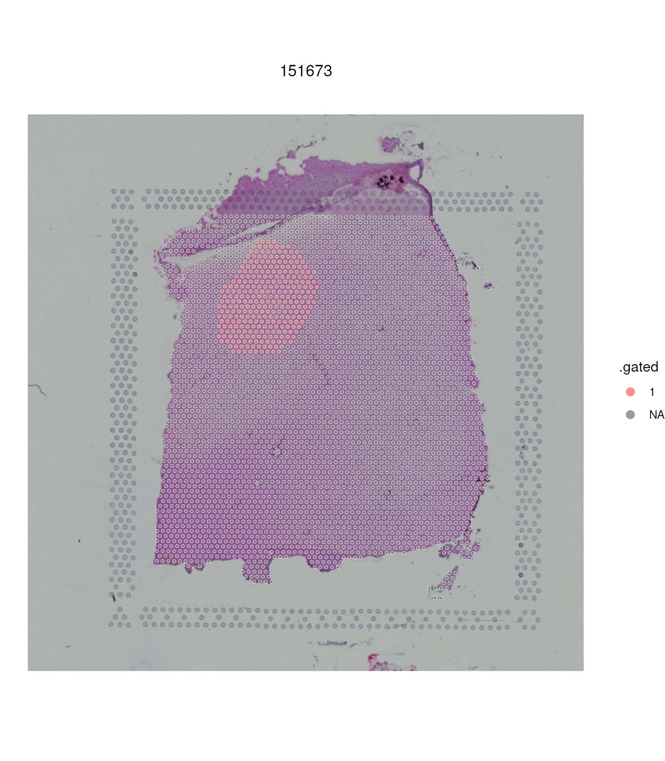

We can also filter, for further analyses

spatial_data |> 
  filter(.gated == 1)

## # A SpatialExperiment-tibble abstraction: 302 × 77
## # Features = 33538 | Cells = 302 | Assays = counts, logcounts
##    .cell      sample_subject sample_id Cluster sum_umi sum_gene subject position
##    <chr>      <chr>          <chr>       <int>   <dbl>    <int> <chr>   <chr>   
##  1 AAAGACCCA… 151673_Br8100  151673          4    4333     2160 Br8100  0       
##  2 AAAGGGCAG… 151673_Br8100  151673          1    2583     1380 Br8100  0       
##  3 AAAGTCACT… 151673_Br8100  151673          2    4858     2352 Br8100  0       
##  4 AACCATGGG… 151673_Br8100  151673          4    3151     1714 Br8100  0       
##  5 AACCCAGAG… 151673_Br8100  151673          4    3878     2113 Br8100  0       
##  6 AACGATAGA… 151673_Br8100  151673          2    4407     2188 Br8100  0       
##  7 AACGTCAGA… 151673_Br8100  151673          2    3066     1775 Br8100  0       
##  8 AACTGGTGT… 151673_Br8100  151673          7    4138     2084 Br8100  0       
##  9 AAGGCGCGT… 151673_Br8100  151673          1    2662     1483 Br8100  0       
## 10 AAGTAGAAG… 151673_Br8100  151673          5    6235     2885 Br8100  0       
## # ℹ 292 more rows
## # ℹ 69 more variables: replicate <chr>, subject_position <chr>, discard <lgl>,
## #   key <chr>, cell_count <int>, SNN_k50_k4 <int>, SNN_k50_k5 <int>,
## #   SNN_k50_k6 <int>, SNN_k50_k7 <int>, SNN_k50_k8 <int>, SNN_k50_k9 <int>,
## #   SNN_k50_k10 <int>, SNN_k50_k11 <int>, SNN_k50_k12 <int>, SNN_k50_k13 <int>,
## #   SNN_k50_k14 <int>, SNN_k50_k15 <int>, SNN_k50_k16 <int>, SNN_k50_k17 <int>,
## #   SNN_k50_k18 <int>, SNN_k50_k19 <int>, SNN_k50_k20 <int>, …

Exercise 2.1 Gate roughly the white matter layer of the tissue (bottom-left) and visualise in UMAP reduced dimensions where this manual gate is distributed.

Calculate PCA, UMAPs as we did for Session 1
Gate the area of white matter
Plot UMAP dimensions according to the gating

4. Work with features

By default tidySpatialExperiment (as well as tidySingleCellExperiment) focus their tidy abstraction on pixels and cells, as this is the key analysis and visualisation unit in spatial and single-cell data. This has proven to be a practical solution to achieve elegant tidy analyses and visualisation.

In contrast, bulk data focuses to features/genes for analysis. In this case its tidy representation with tidySummarizedExperiment prioritise features, exposing them to the user.

If you want to interact with features, the method join_features will be helpful. For example, we can add one or more features of interest to our abstraction.

Let’s add the astrocyte marker GFAP

Find out ENSEMBL ID

rowData(spatial_data) |> 
  as_tibble() |> 
  filter( gene_name == "GFAP")

## # A tibble: 1 × 9
##   source         type  gene_id   gene_version gene_name gene_source gene_biotype
##   <fct>          <fct> <chr>     <chr>        <chr>     <chr>       <chr>       
## 1 ensembl_havana gene  ENSG0000… 12           GFAP      ensembl_ha… protein_cod…
## # ℹ 2 more variables: gene_search <chr>, is_top_hvg <lgl>

Join the feature to the metadata

spatial_data = 
  spatial_data |> 
  join_features("ENSG00000131095", shape="wide")

spatial_data |> 
  select(.cell, ENSG00000131095)

## # A SpatialExperiment-tibble abstraction: 3,639 × 5
## # Features = 33538 | Cells = 3639 | Assays = counts, logcounts
##    .cell         ENSG00000131095 sample_id pxl_col_in_fullres pxl_row_in_fullres
##    <chr>                   <dbl> <chr>                  <dbl>              <dbl>
##  1 AAACAAGTATCT…            0    151673                  9791               8468
##  2 AAACAATCTACT…            3.39 151673                  5769               2807
##  3 AAACACCAATAA…            4.18 151673                  4068               9505
##  4 AAACAGAGCGAC…            0    151673                  9271               4151
##  5 AAACAGCTTTCA…            0    151673                  3393               7583
##  6 AAACAGGGTCTA…            1.83 151673                  3665               8064
##  7 AAACAGTGTTCC…            3.94 151673                  5709              11194
##  8 AAACATTTCCCG…            0    151673                  9437               9783
##  9 AAACCCGAACGA…            1.02 151673                 10690               7875
## 10 AAACCGGGTAGG…            1.86 151673                  4703               7473
## # ℹ 3,629 more rows

Exercise 2.2 Join the endothelial marker PECAM1 (CD31, look for ENSEMBL ID), and plot in space the pixel that are in the 0.75 percentile of EPCAM1 expression. Are the PECAM1-positive pixels (endothelial?) spatially clustered?

Get the ENSEMBL ID
Join the feature to the tidy data abstraction
Calculate the 0.75 quantile across all pixels mutate()
Label the cells with high PECAM1
Plot the slide colouring for the new label

5. Summarisation/aggregation

Distinct

We can quickly explore the elements of a variable with distinct

spatial_data |> 
  distinct(sample_id)

## tidySingleCellExperiment says: A data frame is returned for independent data analysis.

## # A tibble: 1 × 1
##   sample_id
##   <chr>    
## 1 151673

We can distinct across multiple variables

spatial_data |> 
  distinct(sample_id, Cluster)

## tidySingleCellExperiment says: A data frame is returned for independent data analysis.

## # A tibble: 8 × 2
##   sample_id Cluster
##   <chr>       <int>
## 1 151673          7
## 2 151673          4
## 3 151673          8
## 4 151673          6
## 5 151673          3
## 6 151673          5
## 7 151673          1
## 8 151673          2

Count

We can gather more information counting the instances of a variable

spatial_data |> 
  count(Cluster) |> 
  arrange(desc(n))

## tidySingleCellExperiment says: A data frame is returned for independent data analysis.

## # A tibble: 8 × 2
##   Cluster     n
##     <int> <int>
## 1       1   768
## 2       2   597
## 3       3   467
## 4       4   413
## 5       5   372
## 6       6   362
## 7       7   340
## 8       8   320

We calculate summary statistics of a subset of data

spatial_data |> 
filter(Cluster==1) |> 
  count(sample_id) |> 
  arrange(desc(n))

## tidySingleCellExperiment says: A data frame is returned for independent data analysis.

## # A tibble: 1 × 2
##   sample_id     n
##   <chr>     <int>
## 1 151673      768

Aggregate

For summarised analyses, we can aggregate pixels/cells as pseudobulk with the function aggregate_cells. This also works for SingleCellExeriment.We obtain a SummarizedExperiment.

spe_regions_aggregated <-
  spatial_data |>
  aggregate_cells(c(sample_id, spatialLIBD))

spe_regions_aggregated

## class: SummarizedExperiment 
## dim: 33538 8 
## metadata(0):
## assays(2): counts logcounts
## rownames(33538): ENSG00000000003 ENSG00000000005 ... ENSG00000285509
##   ENSG00000285513
## rowData names(1): feature
## colnames(8): 151673___L1 151673___L2 ... 151673___NA 151673___WM
## colData names(16): sample_id spatialLIBD ... file_path
##   sample_id_from_file_path

tidyomics allows to cross spatial, single-cell (Bioconductor and seurat), and bulk keeping a consistent interface.

library(tidySummarizedExperiment)

## 
## Attaching package: 'tidySummarizedExperiment'

## The following object is masked from 'package:tidySingleCellExperiment':
## 
##     tidy

## The following object is masked from 'package:generics':
## 
##     tidy

spe_regions_aggregated

## # A SummarizedExperiment-tibble abstraction: 268,304 × 21
## # Features=33538 | Samples=8 | Assays=counts, logcounts
##    .feature     .sample counts logcounts sample_id spatialLIBD .aggregated_cells
##    <chr>        <chr>    <dbl>     <dbl> <chr>     <fct>                   <int>
##  1 ENSG0000000… 151673…      4      6.06 151673    L1                        273
##  2 ENSG0000000… 151673…      0      0    151673    L1                        273
##  3 ENSG0000000… 151673…     15     20.6  151673    L1                        273
##  4 ENSG0000000… 151673…      3      3.24 151673    L1                        273
##  5 ENSG0000000… 151673…      0      0    151673    L1                        273
##  6 ENSG0000000… 151673…      1      2.01 151673    L1                        273
##  7 ENSG0000000… 151673…      7      9.46 151673    L1                        273
##  8 ENSG0000000… 151673…     11     15.4  151673    L1                        273
##  9 ENSG0000000… 151673…     10     13.9  151673    L1                        273
## 10 ENSG0000000… 151673…      6      9.65 151673    L1                        273
## # ℹ 40 more rows
## # ℹ 14 more variables: sample_subject <chr>, subject <chr>, position <chr>,
## #   replicate <chr>, subject_position <chr>, layer_guess <fct>,
## #   layer_guess_reordered <fct>, layer_guess_reordered_short <fct>,
## #   ManualAnnotation <chr>, in_tissue <lgl>, spatialLIBD_lower <chr>,
## #   file_path <glue>, sample_id_from_file_path <chr>, feature <chr>

You will be able to apply the familiar tidyverse operations

spe_regions_aggregated |> 
  filter(sample_id == "151673")

## # A SummarizedExperiment-tibble abstraction: 268,304 × 21
## # Features=33538 | Samples=8 | Assays=counts, logcounts
##    .feature     .sample counts logcounts sample_id spatialLIBD .aggregated_cells
##    <chr>        <chr>    <dbl>     <dbl> <chr>     <fct>                   <int>
##  1 ENSG0000000… 151673…      4      6.06 151673    L1                        273
##  2 ENSG0000000… 151673…      0      0    151673    L1                        273
##  3 ENSG0000000… 151673…     15     20.6  151673    L1                        273
##  4 ENSG0000000… 151673…      3      3.24 151673    L1                        273
##  5 ENSG0000000… 151673…      0      0    151673    L1                        273
##  6 ENSG0000000… 151673…      1      2.01 151673    L1                        273
##  7 ENSG0000000… 151673…      7      9.46 151673    L1                        273
##  8 ENSG0000000… 151673…     11     15.4  151673    L1                        273
##  9 ENSG0000000… 151673…     10     13.9  151673    L1                        273
## 10 ENSG0000000… 151673…      6      9.65 151673    L1                        273
## # ℹ 40 more rows
## # ℹ 14 more variables: sample_subject <chr>, subject <chr>, position <chr>,
## #   replicate <chr>, subject_position <chr>, layer_guess <fct>,
## #   layer_guess_reordered <fct>, layer_guess_reordered_short <fct>,
## #   ManualAnnotation <chr>, in_tissue <lgl>, spatialLIBD_lower <chr>,
## #   file_path <glue>, sample_id_from_file_path <chr>, feature <chr>

6. tidyfying your workflow

We will take workflow used in Session 2, performed using mostly base R syntax and convert it to tidy R syntax. We will show you how the readability and modularity of your workflow will improve.

Subset to keep only on-tissue spots.

Base R approach:

spatial_data <- spatial_data[, colData(spatial_data)$in_tissue == 1]

Tidyverse Approach:

spatial_data <- 
  spatial_data |> 
  filter(in_tissue == 1)

Specific Differences and Advantages:

The tidyverse filter() function clearly states the intent to filter the dataset, whereas the Base R approach uses subsetting which might not be immediately clear to someone unfamiliar with the syntax.

The tidyverse approach inherently supports chaining further operations without manually checking dimensions, assuming that users trust the operation to behave as expected.

Manipulating feature information

For SingleCellExperiment there is no tidy API for manipulating feature wise data yet, on the contrary for SummarizedExperiment, because gene-centric the abstraction allow for direct gene information manipulation. Currently, tidySingleCellExperiment and tidySpatialExperiment do not prioritize the manipulation of features (genes).

While these functions can employ genes for cell manipulation and visualisation, as demonstrated in join_features(), they lack tools for altering feature-related information. Instead, their primary focus is on cell information, which serves as the main observational unit in single-cell data. This contrasts with bulk RNA sequencing data, where features are more central.

The tidy API for SingleCellExperiment has feature-manipulation API among our plans. See tidyomics challenges

Base R approach:

is_gene_mitochondrial <- grepl("(^MT-)|(^mt-)", rowData(spatial_data)$gene_name)
rowData(spatial_data)$gene_name[is_gene_mitochondrial]

##  [1] "MT-ND1"  "MT-ND2"  "MT-CO1"  "MT-CO2"  "MT-ATP8" "MT-ATP6" "MT-CO3" 
##  [8] "MT-ND3"  "MT-ND4L" "MT-ND4"  "MT-ND5"  "MT-ND6"  "MT-CYB"

Quality Control:

Apply quality control measures to exclude cells based on mitochondrial content and read/gene count, a common indicator of cell health and viability.

Base R approach:

spatial_data <- addPerCellQC(spatial_data, subsets = list(mito = is_gene_mitochondrial))

## Select expressed genes threshold
qc_mitochondrial_transcription <- colData(spatial_data)$subsets_mito_percent > 30
colData(spatial_data)$qc_mitochondrial_transcription <- qc_mitochondrial_transcription

Tidyverse Approach:

spatial_data <- 
  spatial_data |> 
  
  # Add QC
  addPerCellQC(subsets = list(mito = is_gene_mitochondrial)) |> 
  
  ## Add threshold in colData
  mutate(
    qc_mitochondrial_transcription = subsets_mito_percent > 30
  )

spatial_data |> select(.cell, qc_mitochondrial_transcription)

## # A SpatialExperiment-tibble abstraction: 3,639 × 5
## # Features = 33538 | Cells = 3639 | Assays = counts, logcounts
##    .cell  qc_mitochondrial_tra…¹ sample_id pxl_col_in_fullres pxl_row_in_fullres
##    <chr>  <lgl>                  <chr>                  <dbl>              <dbl>
##  1 AAACA… FALSE                  151673                  9791               8468
##  2 AAACA… FALSE                  151673                  5769               2807
##  3 AAACA… FALSE                  151673                  4068               9505
##  4 AAACA… FALSE                  151673                  9271               4151
##  5 AAACA… FALSE                  151673                  3393               7583
##  6 AAACA… FALSE                  151673                  3665               8064
##  7 AAACA… FALSE                  151673                  5709              11194
##  8 AAACA… FALSE                  151673                  9437               9783
##  9 AAACC… FALSE                  151673                 10690               7875
## 10 AAACC… FALSE                  151673                  4703               7473
## # ℹ 3,629 more rows
## # ℹ abbreviated name: ¹qc_mitochondrial_transcription

Specific Differences and Advantages:

tidyverse pipelines these operations without storing intermediate results, directly updating the dataset. Base R separates these steps, requiring manual tracking of variables and updating the dataset in multiple steps, increasing complexity and potential for errors.

Direct Data Mutation: Tidyverse directly mutates the dataset within the pipeline, whereas Base R extracts, computes, and then reassigns values, which can be more verbose and less efficient in terms of workflow clarity and execution.

Group-specific analyses

Base R approach:

# get gene for subset
genes <- !grepl(pattern = "^Rp[l|s]|Mt", x = rownames(spatial_data))

# Convert to list
spatial_data_list <- lapply(unique(spatial_data$sample_id), function(x) spatial_data[, spatial_data$sample_id == x])

# Detect sample-specific hughly-variable genes
marker_genes = 
  lapply( spatial_data_list,
          function(x){
            dec = scran::modelGeneVar(x, subset.row = genes)
            scran::getTopHVGs(dec, n = 1000)
          }
  ) 

head(unique(unlist(marker_genes)))

Tidyverse Approach: group_split

# get gene for subset
genes <- !grepl(pattern = "^Rp[l|s]|Mt", x = rownames(spatial_data))

marker_genes = 
  spatial_data |> 

  # Grouping
  group_split(sample_id) |> 

  # Loop across the list elements
  map(~ .x |> 
      scran::modelGeneVar(subset.row = genes) |> 
      scran::getTopHVGs(n = 1000)
  ) |> 
  reduce(union)

marker_genes |> head()

## [1] "ENSG00000123560" "ENSG00000197971" "ENSG00000110484" "ENSG00000131095"
## [5] "ENSG00000109846" "ENSG00000173786"

Tidyverse Approach: nest

spatial_data |> 
  nest(sample_data = -sample_id) |> 
  mutate(marker_genes = map(sample_data, ~ 
    .x |> 
      scran::modelGeneVar(subset.row = genes) |> 
      scran::getTopHVGs(n = 1000)
  ))

## # A tibble: 1 × 3
##   sample_id sample_data       marker_genes 
##   <chr>     <list>            <list>       
## 1 151673    <SptlExpr[,3639]> <chr [1,000]>

Specific Differences and Advantages:

tidyverse neatly handles grouping and plotting within a single chain, using nest() or group_split() and map() for compartmentalized operations, which organizes the workflow into a coherent sequence.

tidyverse’s map() is a powerful functional language tool, which can return arbitrary types, such as map_int, map_char, map_lgl.It is integrated into the data manipulation workflow, making it part of the data pipeline.

Multi-parameter filtering

Base R approach:

## # Mitochondrial transcription
qc_mitochondrial_transcription <- colData(spatial_data)$subsets_mito_percent > 30
colData(spatial_data)$qc_mitochondrial_transcription <- qc_mitochondrial_transcription

# ## Select library size threshold
qc_total_counts <- colData(spatial_data)$sum < 700
colData(spatial_data)$qc_total_counts <- qc_total_counts

# ## Select expressed genes threshold
qc_detected_genes <- colData(spatial_data)$detected < 500
colData(spatial_data)$qc_detected_genes <- qc_detected_genes

# ## Find combination to filter
colData(spatial_data)$discard <- qc_total_counts | qc_detected_genes | qc_mitochondrial_transcription

# # Filter
spatial_data = spatial_data[,!colData(spatial_data)$discard ]

Tidyverse Approach:

spatial_data_filtered = 
  spatial_data |> 

  mutate(
    discard = 
      subsets_mito_percent > 30 |
      sum < 700 |
      detected < 500
  ) |> 
  filter(!discard)

Specific Differences and Advantages:

Tidyverse: The code directly applies multiple filtering conditions within a single filter() function, making it highly readable and concise. The conditions are clearly laid out, and the operation directly modifies the spatial_data dataframe. This approach is more intuitive for managing complex filters as it condenses them into a singular functional expression.

Base R: The approach first calculates each condition and stores them within the colData of the dataset. These conditions are then combined to create a logical vector that flags rows to discard. Finally, it subsets the data by removing rows that meet any of the discard conditions. This method is more verbose and requires manually handling intermediate logical vectors, which can introduce errors and complexity in tracking multiple data transformations.

Why tidyverse might be better in this context:

Coding efficiency: tidyverse chains operations, reducing the need for intermediate variables and making the code cleaner and less error-prone.

Readability: The filter conditions are all in one place, which simplifies understanding what the code does at a glance, especially for users familiar with the tidyverse syntax.

Maintainability: Fewer and self-explanatory lines of code and no need for intermediate steps make the code easier to maintain and modify, especially when conditions change or additional filters are needed.

7. Visualisation

Here, we will show how to use ad-hoc spatial visualisation, as well as ggplot to explore spatial data we will show how tidySpatialExperiment allowed to alternate between tidyverse visualisation, and any visualisation compatible with SpatialExperiment.

Ad-hoc visualisation: Plotting the regions

Let’s visualise the regions that spatialLIBD labelled across three Visium 10X samples.

spatial_data_filtered |> 
  ggspavis::plotSpots(annotate = "spatialLIBD") +
  facet_wrap(~sample_id) +
  scale_color_manual(values = libd_layer_colors |> str_remove("ayer")) +
  theme(legend.position = "none") +
  labs(title = "spatialLIBD regions")

## Scale for colour is already present.
## Adding another scale for colour, which will replace the existing scale.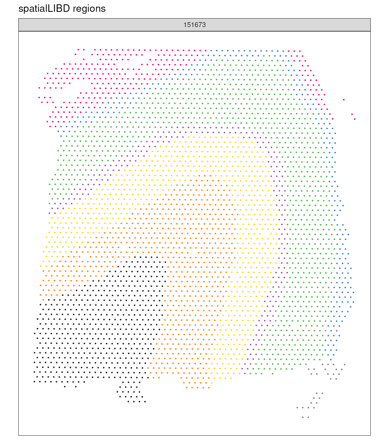

Custom visualisation: Plotting the regions

spatial_data |> 
  ggplot(aes(array_row, array_col)) +
  geom_point(aes(color = spatialLIBD)) +
  facet_wrap(~sample_id) +
  coord_fixed() +
  theme(legend.position = "none") +
  labs(title = "spatialLIBD regions")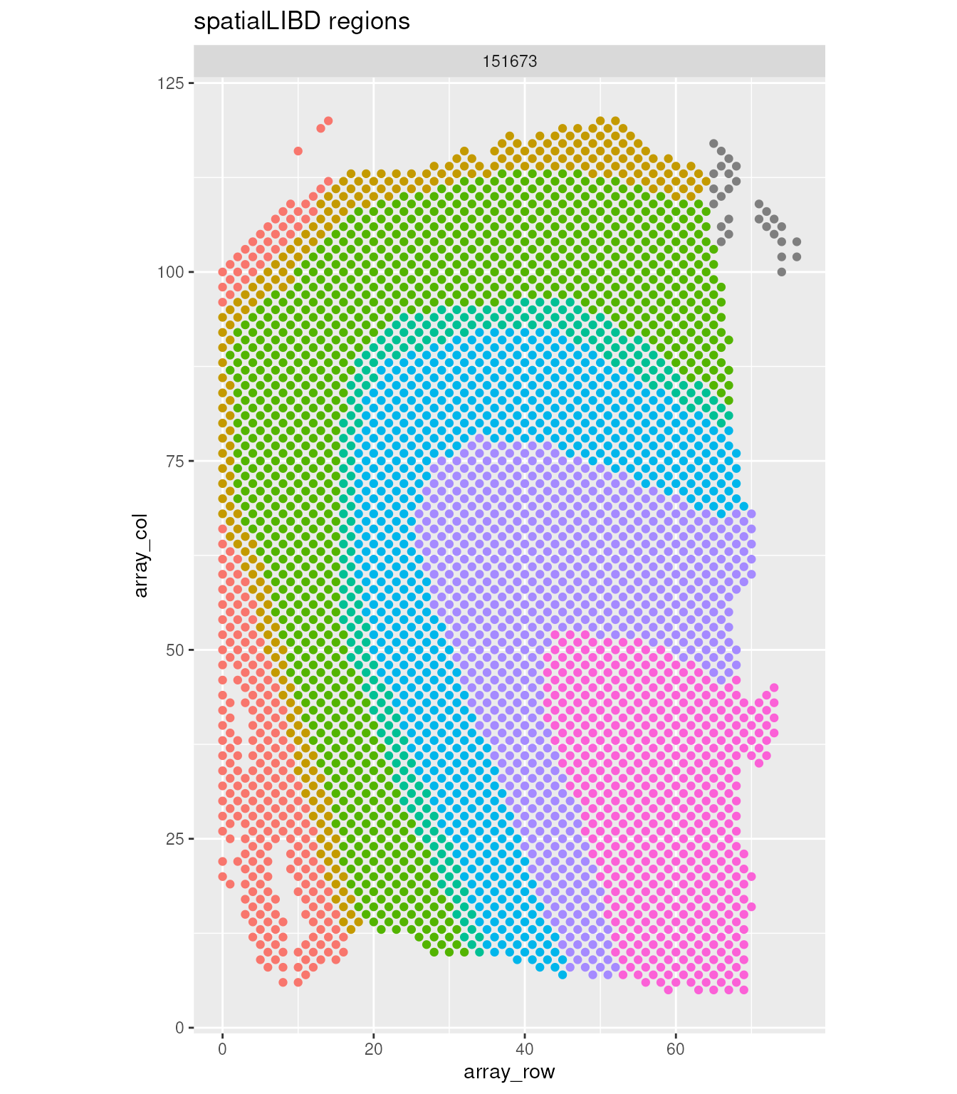

Custom visualisation: Plotting RNA output

Now, let’s observe what is the difference in total transcriptional cell output across regions. We can appreciate that different regions of these Visium slide is characterised by significantly different total RNA output. For example, the region one has a low R&D output, on the contrary regions to an L3, characterised by a high RNA output.

We could conclude that when we use thresholding to filter “low-quality” pixels we have to be careful about possible biological and spatial effects.

spatial_data_filtered |> 
  ggplot(aes(sum_umi, color = spatialLIBD)) +
  geom_density() + 
  facet_wrap(~sample_id) +
  scale_color_manual(values = libd_layer_colors |> str_remove("ayer")) +
  scale_x_log10() +
  theme_bw()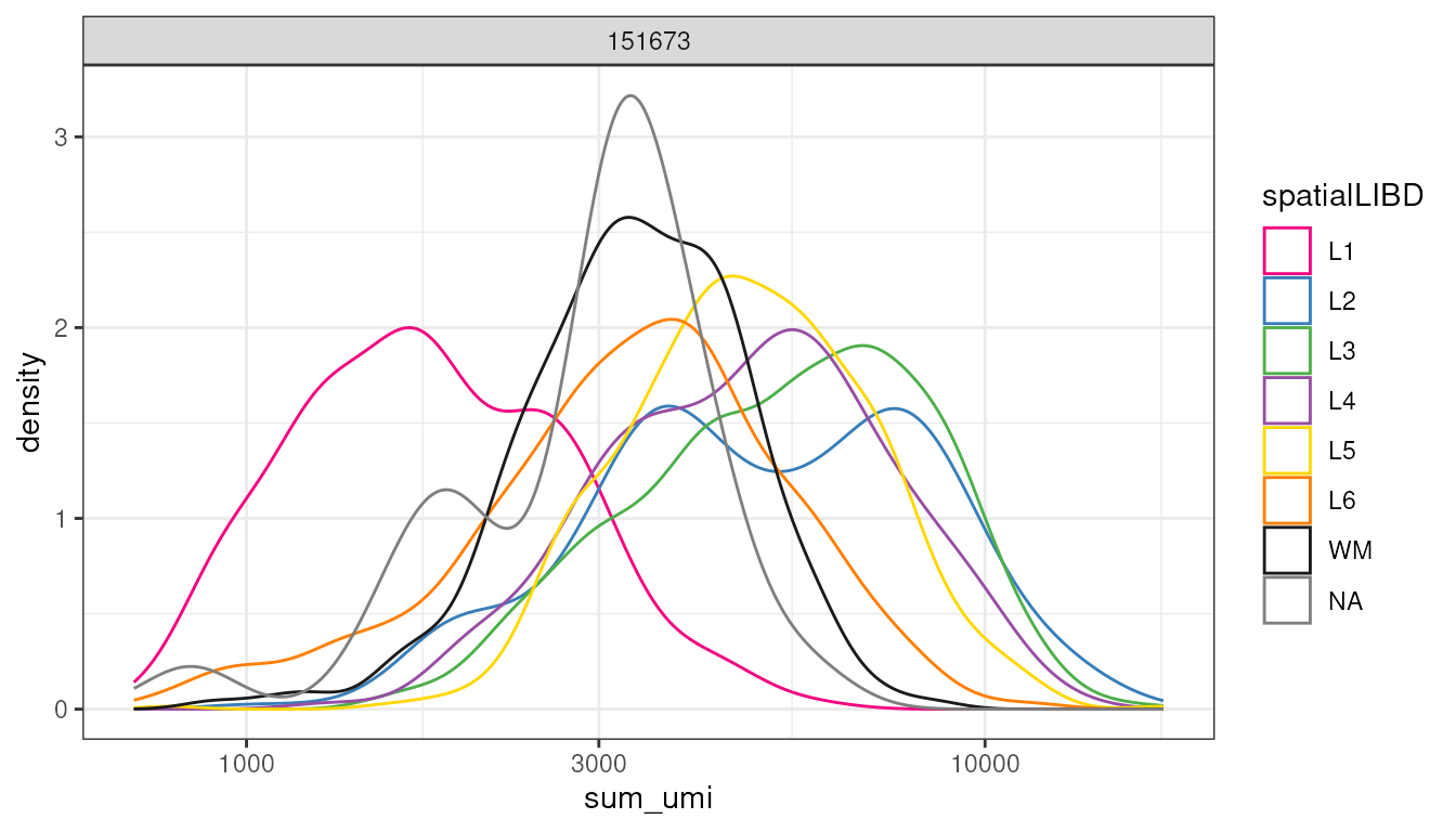

We provide another example of how the use of tidy. Spatial experiment makes custom visualisation, very easy and intuitive, leveraging ggplot functionalities. We will observe the relationship between mitochondrial transcription percentage, and total gene counts. We expect this relationship to be inverse as cells with higher mitochondrial transcription percentage tent to have a more limited transcriptional gene pool (e.g. for dieying or damaged cells).

spatial_data_filtered |> 
  ggplot(aes(subsets_mito_percent, sum_gene)) + 
  geom_point(aes(color = spatialLIBD), size=0.2) +  
  stat_ellipse(aes(group = spatialLIBD), alpha = 0.3) +
  scale_color_manual(values = libd_layer_colors |>
  str_remove("ayer")) +
  scale_y_log10() +
  theme_bw()

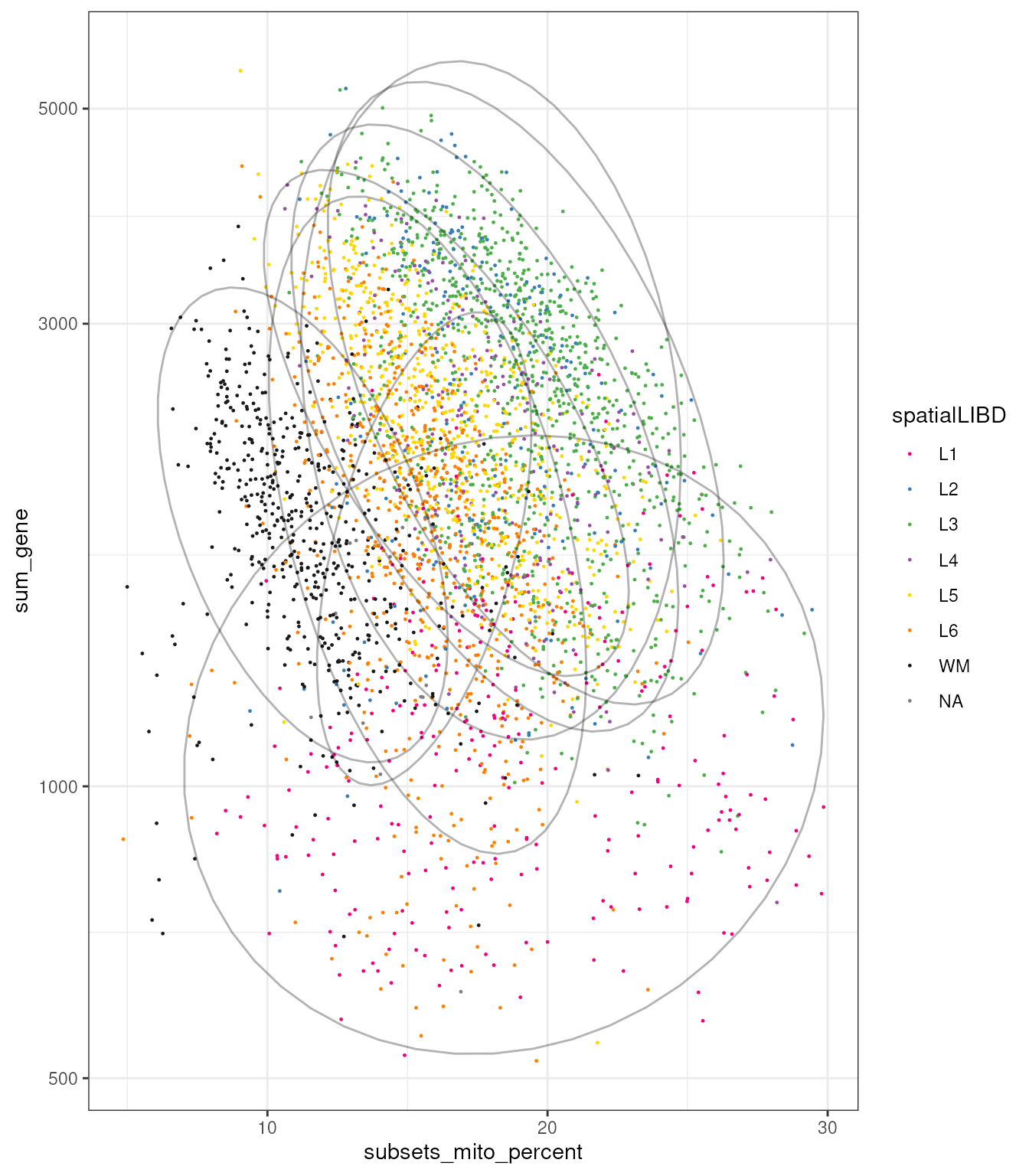
Interestingly, if we plot the correlation between these two quantities we observe heterogeneity among regions, with L1 showing a very small association.

spatial_data_filtered |> 
  ggplot(aes(subsets_mito_percent, sum_gene)) + 
  geom_point(aes(color = spatialLIBD), size=0.2) +  
  scale_color_manual(values = libd_layer_colors |>    str_remove("ayer")) +
  geom_smooth(method="lm") + 
  facet_wrap(~spatialLIBD) + 
  scale_y_log10() +
  theme_bw()

## `geom_smooth()` using formula = 'y ~ x'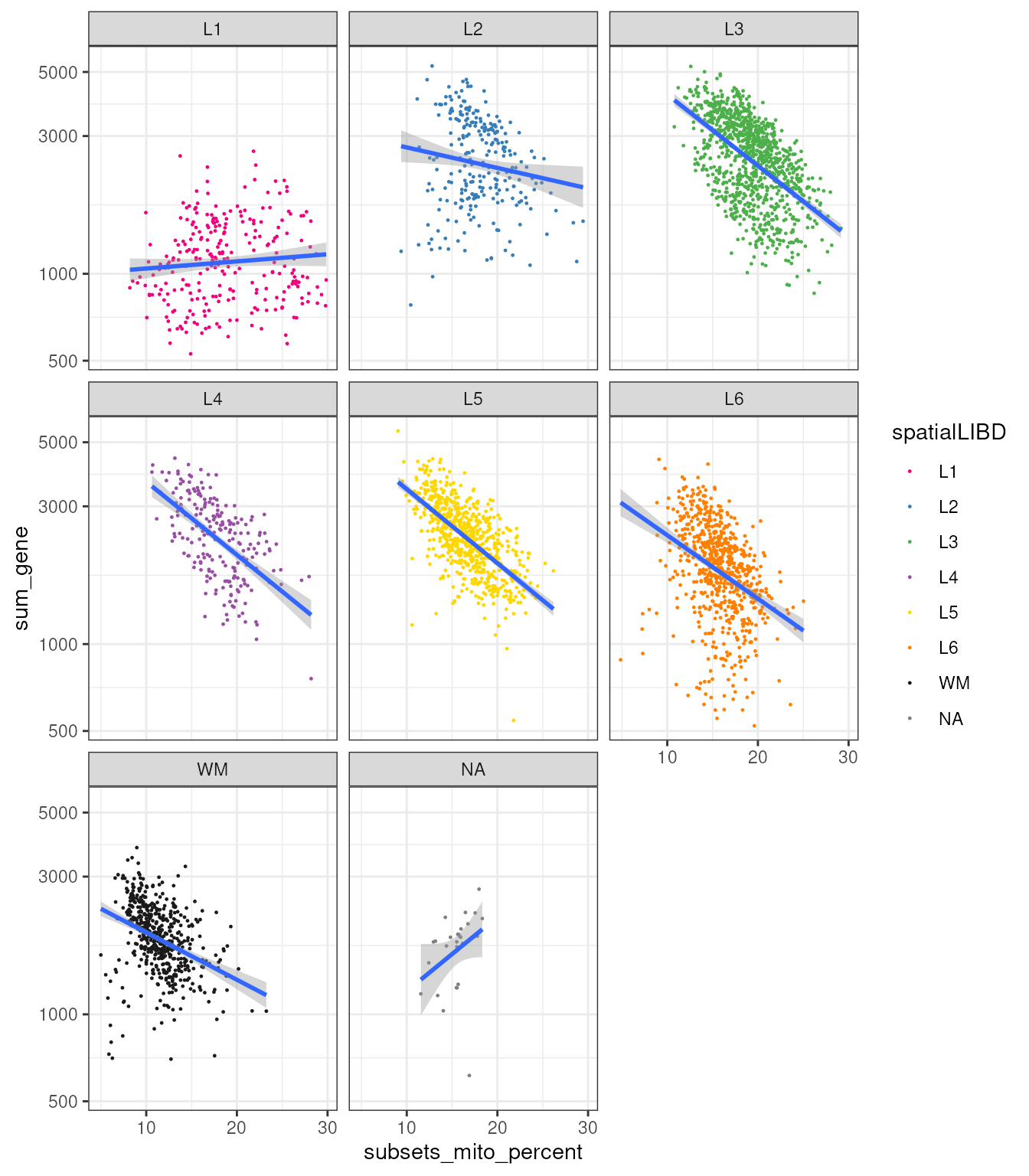

Let’s take a step further and group the correlations according to samples, to see whether different samples show different correlations.

spatial_data_filtered |> 
  ggplot(aes(subsets_mito_percent, sum_gene)) + 
  geom_point(aes(color = spatialLIBD), size=0.2) +  
  scale_color_manual(values = libd_layer_colors |> str_remove("ayer")) +
  geom_smooth(aes(group = sample_id), method="lm") + 
  facet_wrap(~spatialLIBD) + 
  scale_y_log10() +
  theme_bw()

## `geom_smooth()` using formula = 'y ~ x'

As you can appreciate, the relationship between the number of genes, probed Purcell and their mitochondrial prescription abundance it’s quite consistent.

Excercise 2.3 (assisted)

To to practice the use of tidyomics on spatial data, we propose a few exercises that connect manipulation, calculations and visualisation. These exercises are just meant to be simple use cases that exploit tidy R streamlined language.

We assume that the cells we filtered as non-alive or damaged, characterised by being enriched uniquely for mitochondrial, genes, and genes, linked to up apoptosis. It is good practice to check these assumption. This exercise aims to estimate what genes are differentially expressed between filtered and unfiltered cells. Then visualise the results.

Use tidyomic/tidyverse tools to label dead cells and perform differential expression within each region. Some of the comments you can use are: mutate, nest, map, aggregate_cells, tidybulk:::test_differential_abundance,

A hist:

spatial_data |> mutate( dead = …
Aggregate by sample, dead status, ad annotated region
nest by annotated region
use map to test DE

Excercise 2.4

Inspired by our audience, let’s try to use tidyomics to identify potential Amyloid Plaques.

Amyloid plaques are extracellular deposits primarily composed of aggregated amyloid-beta (Aβ) peptides. They are a hallmark of Alzheimer’s disease (AD) and are also found in certain other neurodegenerative conditions.

Amyloid plaques can be found in the brains of mice, particularly in transgenic mouse models that are engineered to develop Alzheimer’s disease-like pathology. Although amyloid plaques themselves are extracellular, the presence and formation of these plaques are associated with specific gene expression changes in the surrounding and involved cells. These gene markers are indicative of the processes that contribute to amyloid plaque formation, as well as the cellular response to these plaques (Ranman et al., 2021.)

join_features()
mutate()
ggspavis::plotSpots()

marker_genes_of_amyloid_plaques = c("APP", "PSEN1", "PSEN2", "CLU", "APOE", "CD68", "ITGAM", "AIF1")

rownames(spatial_data) = rowData(spatial_data)$gene_name

The excercise includes

Join the features
Rescaling
Summarising signature (sum), mutate()
Plotting colousing by the signature :::

Session Information

sessionInfo()

## R version 4.5.0 (2025-04-11)
## Platform: x86_64-pc-linux-gnu
## Running under: Ubuntu 24.04.2 LTS
## 
## Matrix products: default
## BLAS:   /usr/lib/x86_64-linux-gnu/openblas-pthread/libblas.so.3 
## LAPACK: /usr/lib/x86_64-linux-gnu/openblas-pthread/libopenblasp-r0.3.26.so;  LAPACK version 3.12.0
## 
## locale:
##  [1] LC_CTYPE=en_US.UTF-8       LC_NUMERIC=C              
##  [3] LC_TIME=en_US.UTF-8        LC_COLLATE=en_US.UTF-8    
##  [5] LC_MONETARY=en_US.UTF-8    LC_MESSAGES=en_US.UTF-8   
##  [7] LC_PAPER=en_US.UTF-8       LC_NAME=C                 
##  [9] LC_ADDRESS=C               LC_TELEPHONE=C            
## [11] LC_MEASUREMENT=en_US.UTF-8 LC_IDENTIFICATION=C       
## 
## time zone: Etc/UTC
## tzcode source: system (glibc)
## 
## attached base packages:
## [1] stats4    stats     graphics  grDevices utils     datasets  methods  
## [8] base     
## 
## other attached packages:
##  [1] tidySummarizedExperiment_1.19.0 tidySpatialExperiment_1.5.0    
##  [3] ttservice_0.4.1                 tidySingleCellExperiment_1.19.0
##  [5] ExperimentHub_2.99.0            AnnotationHub_3.99.1           
##  [7] BiocFileCache_2.99.0            dbplyr_2.5.0                   
##  [9] spatialLIBD_1.21.4              scran_1.37.0                   
## [11] scater_1.37.0                   scuttle_1.19.0                 
## [13] ggspavis_1.15.0                 dittoSeq_1.21.0                
## [15] colorspace_2.1-1                stringr_1.5.1                  
## [17] glue_1.8.0                      purrr_1.0.4                    
## [19] tidyr_1.3.1                     dplyr_1.1.4                    
## [21] plotly_4.10.4                   ggplot2_3.5.2                  
## [23] SpatialExperiment_1.19.0        SingleCellExperiment_1.31.0    
## [25] SummarizedExperiment_1.39.0     Biobase_2.69.0                 
## [27] GenomicRanges_1.61.0            GenomeInfoDb_1.45.3            
## [29] IRanges_2.43.0                  S4Vectors_0.47.0               
## [31] BiocGenerics_0.55.0             generics_0.1.3                 
## [33] MatrixGenerics_1.21.0           matrixStats_1.5.0              
## [35] here_1.0.1                     
## 
## loaded via a namespace (and not attached):
##   [1] splines_4.5.0              later_1.4.2               
##   [3] BiocIO_1.19.0              bitops_1.0-9              
##   [5] filelock_1.0.3             tibble_3.2.1              
##   [7] XML_3.99-0.18              tidySpatialWorkshop_0.18.5
##   [9] lifecycle_1.0.4            httr2_1.1.2               
##  [11] edgeR_4.7.2                doParallel_1.0.17         
##  [13] rprojroot_2.0.4            MASS_7.3-65               
##  [15] lattice_0.22-7             magrittr_2.0.3            
##  [17] limma_3.65.0               sass_0.4.10               
##  [19] rmarkdown_2.29             jquerylib_0.1.4           
##  [21] yaml_2.3.10                metapod_1.17.0            
##  [23] httpuv_1.6.16              ggside_0.3.1              
##  [25] sessioninfo_1.2.3          cowplot_1.1.3             
##  [27] DBI_1.2.3                  RColorBrewer_1.1-3        
##  [29] golem_0.5.1                abind_1.4-8               
##  [31] RCurl_1.98-1.17            rappdirs_0.3.3            
##  [33] circlize_0.4.16            ggrepel_0.9.6             
##  [35] irlba_2.3.5.1              pheatmap_1.0.12           
##  [37] dqrng_0.4.1                pkgdown_2.1.2             
##  [39] codetools_0.2-20           DelayedArray_0.35.1       
##  [41] DT_0.33                    tidyselect_1.2.1          
##  [43] shape_1.4.6.1              UCSC.utils_1.5.0          
##  [45] farver_2.1.2               ScaledMatrix_1.17.0       
##  [47] viridis_0.6.5              shinyWidgets_0.9.0        
##  [49] GenomicAlignments_1.45.0   jsonlite_2.0.0            
##  [51] GetoptLong_1.0.5           BiocNeighbors_2.3.0       
##  [53] ellipsis_0.3.2             ggridges_0.5.6            
##  [55] iterators_1.0.14           systemfonts_1.2.3         
##  [57] foreach_1.5.2              tools_4.5.0               
##  [59] ragg_1.4.0                 Rcpp_1.0.14               
##  [61] gridExtra_2.3              SparseArray_1.9.0         
##  [63] mgcv_1.9-3                 xfun_0.52                 
##  [65] withr_3.0.2                BiocManager_1.30.25       
##  [67] fastmap_1.2.0              fansi_1.0.6               
##  [69] bluster_1.19.0             digest_0.6.37             
##  [71] rsvd_1.0.5                 R6_2.6.1                  
##  [73] mime_0.13                  textshaping_1.0.1         
##  [75] RSQLite_2.3.11             config_0.3.2              
##  [77] utf8_1.2.5                 data.table_1.17.0         
##  [79] rtracklayer_1.69.0         httr_1.4.7                
##  [81] htmlwidgets_1.6.4          S4Arrays_1.9.0            
##  [83] pkgconfig_2.0.3            gtable_0.3.6              
##  [85] blob_1.2.4                 ComplexHeatmap_2.25.0     
##  [87] XVector_0.49.0             htmltools_0.5.8.1         
##  [89] clue_0.3-66                scales_1.4.0              
##  [91] png_0.1-8                  attempt_0.3.1             
##  [93] knitr_1.50                 rjson_0.2.23              
##  [95] nlme_3.1-168               curl_6.2.2                
##  [97] cachem_1.1.0               GlobalOptions_0.1.2       
##  [99] BiocVersion_3.22.0         parallel_4.5.0            
## [101] vipor_0.4.7                AnnotationDbi_1.71.0      
## [103] restfulr_0.0.15            desc_1.4.3                
## [105] pillar_1.10.2              grid_4.5.0                
## [107] vctrs_0.6.5                promises_1.3.2            
## [109] BiocSingular_1.25.0        beachmat_2.25.0           
## [111] xtable_1.8-4               cluster_2.1.8.1           
## [113] beeswarm_0.4.0             paletteer_1.6.0           
## [115] evaluate_1.0.3             magick_2.8.6              
## [117] Rsamtools_2.25.0           cli_3.6.5                 
## [119] locfit_1.5-9.12            compiler_4.5.0            
## [121] rlang_1.1.6                crayon_1.5.3              
## [123] labeling_0.4.3             rematch2_2.1.2            
## [125] fs_1.6.6                   ggbeeswarm_0.7.2          
## [127] stringi_1.8.7              viridisLite_0.4.2         
## [129] BiocParallel_1.43.0        Biostrings_2.77.0         
## [131] lazyeval_0.2.2             Matrix_1.7-3              
## [133] benchmarkme_1.0.8          bit64_4.6.0-1             
## [135] KEGGREST_1.49.0            statmod_1.5.0             
## [137] shiny_1.10.0               tidygate_1.0.14           
## [139] igraph_2.1.4               memoise_2.0.1             
## [141] bslib_0.9.0                benchmarkmeData_1.0.4     
## [143] bit_4.6.0

References

mangiola.stefano@adelaide.edu.au ↩︎
<mangiola.s at wehi.edu.au>↩︎

Stefano Mangiola, South Australian immunoGENomics Cancer Institute1, Walter and Eliza Hall Institute2

Session 2: Tidying spatial data

Introduction to tidyomics

Installation

Working with tidySpatialExperiment

1. tidySpatialExperiment package

Data interface, display

Original behaviour is preserved

2. Tidyverse commands

Select

Filter

Summarise

Mutate

Extract

Unite

3. Advanced filtering/gating and pseudobulk

4. Work with features

5. Summarisation/aggregation

Distinct

Count

Aggregate

6. tidyfying your workflow

Subset to keep only on-tissue spots.

Manipulating feature information

Quality Control:

Group-specific analyses

Multi-parameter filtering

7. Visualisation

Ad-hoc visualisation: Plotting the regions

Custom visualisation: Plotting the regions

Custom visualisation: Plotting RNA output

Stefano Mangiola, South Australian immunoGENomics Cancer Institute¹, Walter and Eliza Hall Institute²